Efficient Image Compression Techniques: Balancing Data and Information Preservation
Learn about the trade-offs between lossless and lossy image compression, reducing redundancy types, coding schemes, interpixel redundancy, and psychovisual factors in image compression. Explore how to measure information content and estimate redundancy for optimal compression ratios.

Efficient Image Compression Techniques: Balancing Data and Information Preservation
E N D
Presentation Transcript
Image Compression CS474/674 – Prof. Bebis Chapter 8 (except Sections 8.10-8.12)
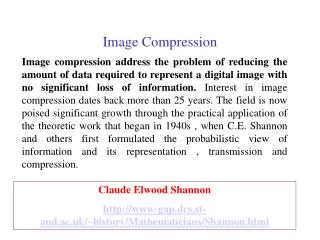
Image Compression • The goal of image compression is to reduce the amount of data required to represent a digital image.
Image Compression (cont’d) • Lossless • Information preserving • Low compression ratios • Lossy • Information loss • High compression ratios Trade-off: information loss vscompression ratio
Data ≠ Information • Data and information are not synonymous terms! • Datais the means by which information is conveyed. Goal of data compression Reduce the amount of data while preserving as much information as possible!
Data vs Information (cont’d) • The same information can be represented by different amount of data – for example: Ex1: Your wife, Helen, will meet you at Logan Airport in Boston at 5 minutes past 6:00 pm tomorrow night Your wife will meet you at Logan Airport at 5 minutes past 6:00 pm tomorrow night Helen will meet you at Logan at 6:00 pm tomorrow night Ex2: Ex3:
Compression Ratio compression Compression ratio:
Relevant Data Redundancy Example:
Types of Data Redundancy (1) Coding Redundancy (2) InterpixelRedundancy (3) PsychovisualRedundancy • Data compression attempts to reduce one or more of these redundancy types.
Coding Redundancy Code: a list of symbols (letters, numbers, bits etc.) Code word: a sequence of symbols used to represent some information (e.g., gray levels). Code word length: number of symbols in a code word. Could be fixed or variable To reduce coding redundancy, we need efficient coding schemes!
Coding Redundancy (cont’d) • To compare the efficiency of different coding schemes, we need to compute the average number of symbols Lavg per code word. N x M image rk: k-th gray level l(rk):# of bits for rk P(rk):probability of rk Example: Average Image Size:
Coding Redundancy (cont’d) • Case 1: l(rk) = fixed length (code 1) Example:
Coding Redundancy (cont’d) • Case 2: l(rk) = variable length (code 2 – Huffman code) Total number of bits: 2.7NM
Interpixel redundancy • Interpixel redundancy implies that pixel values are correlated (i.e., a pixel value can be reasonably predicted by its neighbors). histograms auto-correlation auto-correlation: f(x)=g(x)
Interpixel redundancy (cont’d) • To reduce interpixel redundancy, some kind of a transformation must be applied on the data. Example Additional savings using run-length coding Original threshold threshold 11 ……………0000……………………..11…..000….. Binary image (1+10) bits/pair
Psychovisual redundancy • The human eye is more sensitive to the lower frequencies than to the higher frequencies in the visual spectrum. • Idea: discard data that is perceptually insignificant! 16 gray levels + random noise 256 gray levels 16 gray levels i.e., add a small pseudo-random number to each pixel prior to quantization Example: quantization C=8/4 = 2:1
Measuring Information • The key question in image compression is: • How do we measure the information content of an image? “What is the minimum amount of data that is sufficient to describe completely an image without loss of information?”
Measuring Information (cont’d) • We assume that information generation is a probabilistic process. • Associate information with probability! A random event E withprobability P(E) contains: Note: I(E)=0 when P(E)=1
How much information does a pixel value contain? • Suppose that gray level values are generated by a random process, then rkcontains: units of information! (assuming statistically independent random events)
How much information does an image contain? • Average information content of an image: using units/pixel (e.g., bits/pixel) Entropy:
Redundancy • Redundancy: (data vs info) where: Note: if Lavg= H, then R=0 (no redundancy)
Entropy Estimation • It is not easy to estimate H reliably! image
Entropy Estimation (cont’d) First order estimate of H: What is the redundancy? R= Lavg- H where Lavg = 8 bits/pixel R= 6.19 bits/pixel
Estimating Entropy (cont’d) • Second order estimate of H: • Use relative frequencies of pixel blocks : image
Estimating Entropy (cont’d) • What does it mean that the first- and second-order entropies are different? • In general, differences between first-order and higher-order entropy estimates indicate the presence of interpixel redundancy(i.e., need to apply some transformation).
Differences in Entropy Estimates (cont’d) Example: take pixel differences 16
Differences in Entropy Estimates (cont’d) Example (cont’d): • What is the entropy of the pixel differences image? • An even better transformation should be possible since the second order entropy estimate is lower: (better than the entropy of the original image H=1.81)
Image Compression Model We will focus on the Source Encoder/Decoderonly.
Encoder • Mapper: transforms data to account for interpixel redundancies.
Encoder (cont’d) Quantizer: quantizes the data to account for psychovisual redundancies.
Encoder (cont’d) Symbol encoder:encodes the data to account for coding redundancies.
Decoder • The decoder applies the inverse steps. • Note that the quantization is irreversible in general!
Fidelity Criteria How close is to ? Criteria Subjective: based on human observers Objective:mathematically defined criteria
Objective Fidelity Criteria Root mean square error (RMS) Mean-square signal-to-noise ratio (SNR)
Taxonomy of Lossless Methods (Run-length encoding) (see “Image Compression Techniques” paper)
Huffman Coding (addresses coding redundancy) • A variable-length coding technique. • Source symbols are encoded one at a time! • There is a one-to-one correspondence between source symbols and code words. • Optimal code - minimizes code word length per source symbol.
Huffman Coding (cont’d) • Forward Pass 1. Sort probabilities per symbol 2. Combine the lowest two probabilities 3. Repeat Step2 until only two probabilities remain.
Huffman Coding (cont’d) • Backward Pass Assign code symbols going backwards
Huffman Coding (cont’d) • Lavgassuming binary coding: • Lavgassuming Huffman coding:
Huffman Coding-Decoding • Both coding and decodingcan be implemented using a look-up table. • Note that decoding can be done unambiguously.
Arithmetic (or Range) Coding (addresses coding redundancy) • Huffman coding encodes source symbols one at a time which might not be efficient. • Arithmetic coding encodes sequences of source symbols to variable length code words. • There is no one-to-one correspondence between source symbols and code words. • Slower than Huffman coding but can achieve better compression.
Arithmetic Coding (cont’d) • Main idea: • Map a sequence of symbols to a number (arithmetic code) in the interval [0, 1). • Encoding the arithmetic code is more efficient. • The mapping depends on the probabilities of the symbols. • The mapping is built as each symbol arrives. α1α2α3α3α4
0 0 0 1 1 1 Arithmetic Coding (cont’d) α1α2α3α3α4 • Main idea: • Start with the interval [0, 1) • A sub-interval of [0,1) is chosen to represent the first symbol (based on its probability of occurrence). • As more symbols are encoded, the sub-interval gets smaller and smaller. • At the end, the symbol sequence is encoded by a number within the final interval.
Example Encode α1α2α3α3α4 [0.06752, 0.0688) code: 0.068 (any number within sub-interval) 0.8 0.4 0.2 Warning: finite precision arithmetic might cause problems due to truncations!
Example (cont’d) • The arithmetic code 0.068 can be encoded using Binary Fraction: 0.0068 ≈ 0.000100011 (9 bits) (subject to conversion error; exact value is 0.068359375) • Huffman Code: 0100011001 (10 bits) • Fixed Binary Code: 5 x 8 bits/symbol = 40 bits α1α2α3α3α4
Arithmetic Decoding 1.0 0.8 0.72 0.592 0.5728 α4 0.5856 0.57152 0.8 0.72 0.688 Decode 0.572 α3 0.5728 0.56896 0.4 0.56 0.624 α2 α3α3α1α2α4 0.2 0.48 0.592 0.5664 0.56768 α1 0.0 0.4 0.56 0.56 0.5664
LZW Coding(addresses interpixel redundancy) • Requires no prior knowledge of symbol probabilities. • Assignssequences of source symbols to fixed length code words. • There is no one-to-one correspondence between source symbols and code words. • Included in GIF, TIFF and PDF file formats
Dictionary Location Entry 0 0 1 1 . . 255 255 256 - 511 - LZW Coding • A codebook (or dictionary) needs to be constructed. • Initially, the first 256 entries of the dictionary are assigned to the gray levels 0,1,2,..,255 (i.e., assuming 8 bits/pixel) Initial Dictionary
Dictionary Location Entry 0 0 1 1 . . 255 255 256 - 511 - LZW Coding (cont’d) Example: As the encoder examines image pixels, gray level sequences (i.e., blocks) that are not in the dictionary are assigned to a new entry. 39 39 126 126 39 39 126 126 39 39 126 126 39 39 126 126 - Is 39 in the dictionary……..Yes - What about 39-39………….No * Add 39-39 at location 256 39-39