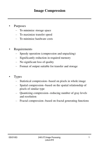
Image Compression
Image Compression. Roger Cheng (JPEG slides courtesy of Brian Bailey) Spring 2007. Ubiquitous use of digital images. Goal. Store image data as efficiently as possible Ideally, want to Maximize image quality Minimize storage space and processing resources Can’t have best of both worlds

Image Compression
E N D
Presentation Transcript
Image Compression Roger Cheng (JPEG slides courtesy of Brian Bailey) Spring 2007
Goal • Store image data as efficiently as possible • Ideally, want to • Maximize image quality • Minimize storage space and processing resources • Can’t have best of both worlds • What are some good compromises?
Digital vs. Analog • Modern image processing is done in digital domain • If we have an analog source image, convert it to digital format before doing any processing
Lossless Stored image data can reproduce original image exactly Takes more storage space Uses entropy coding only (or none at all) Examples: BMP, TIFF, GIF Lossy Stored image data can reproduce something that looks “close” to the original image Uses both quantization and entropy coding Usually involves transform into frequency or other domain Examples: JPEG, JPEG-2000 Two main schools of image compression
BMP (Bitmap) • Use 3 bytes per pixel, one each for R, G, and B • Can represent up to 224 = 16.7 million colors • No entropy coding • File size in bytes = 3*length*height, which can be very large • Can use fewer than 8 bits per color, but you need to store the color palette • Performs well with ZIP, RAR, etc.
GIF (Graphics Interchange Format) • Can use up to 256 colors from 24-bit RGB color space • If source image contains more than 256 colors, need to reprocess image to fewer colors • Suitable for simpler images such as logos and textual graphics, not so much for photographs • Uses LZW lossless data compression
JPEG (Joint Photographic Experts Group) • Most dominant image format today • Typical file size is about 10% of that of BMP (can vary depending on quality settings) • Unlike GIF, JPEG is suitable for photographs, not so much for logos and textual graphics
JPEG Encoding Steps • Preprocess image • Apply 2D forward DCT • Quantize DCT coefficients • Apply RLE, then entropy encoding
JPEG Block Diagram 8x8 blocks SourceImage B G R DCT-based encoding Compressedimage data FDCT Quantizer EntropyEncoder Table Table
Preprocess • Shift values [0, 2P - 1] to [-2P-1, 2P-1 - 1] • e.g. if (P=8), shift [0, 255] to [-127, 127] • DCT requires range be centered around 0 • Segment each component into 8x8 blocks • Interleave components (or not) • may be sampled at different rates
Interleaving • Non-interleaved: scan from left to right, top to bottom for each color component • Interleaved: compute one “unit” from each color component, then repeat • full color pixels after each step of decoding • but components may have different resolution
Color Transformation (optional) • Down-sample chrominance components • compress without loss of quality (color space) • e.g., YUV 4:2:2 or 4:1:1 • Example: 640 x 480 RGB to YUV 4:1:1 • Y is 640x480 • U is 160x120 • V is 160x120
Interleaving • ith color component has dimension (xi, yi) • maximum dimension value is 216 • [X, Y] where X=max(xi) and Y=max(yi) • Sampling among components must be integral • Hi and Vi; must be within range [1, 4] • [Hmax, Vmax] where Hmax=max(Hi) and Vmax=max(Vi) • xi = X * Hi / Hmax • yi = Y * Vi / Vmax
Example [Wallace, 1991]
Forward DCT • Convert from spatial to frequency domain • convert intensity function into weighted sum of periodic basis (cosine) functions • identify bands of spectral information that can be thrown away without loss of quality • Intensity values in each color plane often change slowly
Understanding DCT • For example, in R3, we can write (5, 2, 9) as the sum of a set of basis vectors • we know that [(1,0,0), (0,1,0), (0,0,1)] provides one set of basis functions in R3 (5,2,9) = 5*(1,0,0) + 2*(0,1,0) + 9*(0,0,1) • DCT is same process in function domain
DCT Basic Functions • Decompose the intensity function into a weighted sum of cosine basis functions
1D Forward DCT • Given a list of n intensity values I(x),where x = 0, …, N-1 • Compute the N DCT coefficients:
1D Inverse DCT • Given a list of n DCT coefficients F(u),where u = 0, …, n-1 • Compute the n intensity values:
Extend DCT from 1D to 2D • Perform 1D DCT on each row of the block • Again for each column of 1D coefficients • alternatively, transpose the matrix and perform DCT on the rows Y X
Equations for 2D DCT • Forward DCT: • Inverse DCT:
Visualization of Basis Functions Increasing frequency Increasing frequency
Quantization • Divide each coefficient by integer [1, 255] • comes in the form of a table, same size as a block • multiply the block of coefficients by the table, round result to nearest integer • In the decoding process, multiply the quantized coefficients by the inverse of the table • get back a number close to original • error is less than 1/2 of the quantization number • Larger quantization numbers cause more loss
De facto Quantization Table Eye becomes less sensitive Eye becomes less sensitive
Entropy Encoding • Compress sequence of quantized DC and AC coefficients from quantization step • further increase compression, without loss • Separate DC from AC components • DC components change slowly, thus will be encoded using difference encoding
DC Encoding • DC represents average intensity of a block • encode using difference encoding scheme • use 3x3 pattern of blocks • Because difference tends to be near zero, can use less bits in the encoding • categorize difference into difference classes • send the index of the difference class, followed by bits representing the difference
AC Encoding • Use zig-zag ordering of coefficients • orders frequency components from low->high • produce maximal series of 0s at the end • Apply RLE to ordering
Huffman Encoding • Sequence of DC difference indices and values along with RLE of AC coefficients • Apply Huffman encoding to sequence – Exploits sequence’s statistics by assigning frequently used symbols fewer bits than rare symbols • Attach appropriate headers • Finally have the JPEG image!
JPEG Decoding Steps • Basically reverse steps performed in encoding process • Parse compressed image data and perform Huffman decoding to get RLE symbols • Undo RLE to get DCT coefficient matrix • Multiply by the quantization matrix • Take 2-D inverse DCT of this matrix to get reconstructed image data
Reconstruction Error • Resulting image is “close” to original image • Usually measure “closeness” with MSE (Mean Squared Error) and PSNR (Peak Signal to Noise Ratio) – Want low MSE and high PSNR
Analysis • Near perfect image at 2.76M, so-so image at 88K • Sharpness decreases as file size decreases • False contours visible at 144K and 88K • Can be fixed by dithering image before quantization • Which file size is the best? • No correct answer to this question • Answer depends upon how strict we are about image quality, what purpose image is to be used for, and the resources available
Conclusion • Image compression is important • Image compression has come a long way • Image compression is nearly mature, but there is always room for improvement

