Image Compression

1. Image Compression Shinta P.

2. Data Compression System

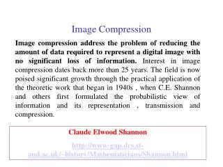
3. Goal of Image Compression • Digital images require huge amounts of space for storage and large bandwidths for transmission. • A 640 x 480 color image requires close to 1MB of space. • The goal of image compression is to reduce the amount of data required to represent a digital image. • Reduce storage requirements and increase transmission rates.

4. Data Compression • Forms of data - text, numerical, image, video contain redundant elements. • Data can be compressed by eliminating the redundant elements. • A code is substituted for the eliminated redundant element, where the code is shorter than eliminated element. • When compressed data is retrieved from storage or received over a communications link, it is expanded back to its original form, based on the code.

5. REDUNDANCY Most types of computer files are fairly redundant they have the same information listed over and over again. File-compression programs simply get rid of the redundancy “Ask not what your country can do for you -- ask what you can do for your country.”

6. Techniques • Lossless • Data can be completely recovered after decompression • Recovered data is identical to original • Exploits redundancy in data • Lossy • Data cannot be completely recovered after decompression • Some information is lost for ever • Gives more compression than lossless • Discards “insignificant” data components

7. Image Compression • Image compression can be lossy or lossless • Methods for lossless image compression are: • Run-length encoding • Entropy coding • Adaptive dictionary algorithms such as LZW • Methods for lossy compression are: • Reducing the color space to the most common colors in the image. The selected colors are specified in the color palette in the header of the compressed image. Each pixel just references the index of a color in the color palette. This method can be combined with dithering to blur the color borders. • Transform coding. This is the most commonly used method. A Fourier-related transform such as DCT or the wavelet transform are applied, followed by quantization and entropy coding.

8. Traditional Evaluation Criteria • Algorithm complexity • running time • Amount of compression • redundancy • compression ratio • How to measure?

9. JPEG • JPEG is named after its origin, the Joint Photographers Experts Group • This involves reducing the number of bits per sample or entirely discard some of the samples

10. MULTIMEDIA COMPRESSION • Multimedia compression is a general term referring to the compression of any type of multimedia, most notably graphics, audio, and video • MPEG (Moving Pictures Experts Group ) The future of this technology is to encode the compression and uncompression algorithms directly into integrated circuits. • The approach used by MPEG can be divided into two types of compression: within-the-frame and between-frame

11. DATA COMPRESSION ALGORITHMS LOSS LESS COMPRESSION Run Length Encoding Huffman Coding LZW LOSSY COMPRESSION JPEG MPEG

12. Compression Principles • Entropy Encoding • Statistical encoding • Based on the probability of occurrence of a pattern • The more probable, the shorter codeword • “Prefix property”: a shorter codeword must not form the start of a longer codeword

13. RUN-LENGTH ENCODING Data files frequently contain the same character repeated many times in a row. Example of run-length encoding. Each run of zeros is replaced by two characters in the compressed file: a zero to indicate that compression is occurring, followed by the number of zeros in the run.

14. Run Length Encoding CTAAAAAGGGTCGTTTTTTGCCCGGGGGCCTCCCCCCC CTAAAAAGGGTCGTTTTTTGCCCGGGGGCCTCCCCCCC CTAAAAAGGGTCGTTTTTTGCCCGGGGGCCTCCCCCCC CT5A3GTCG6TG3C5GCCT7C } Run length encoded: 21 symbols

15. Run Length Encoding (cont.) WWWBWWWWWBWWWBWWWWBWWWWWBWWWBWWWWWBWWBWWWWWWBBBWWWWWWWBWBWWWWWWWBWWBBWWWWWBWWWWBWWWWBWWWWB WWWBWWWWWBWWWBWWWWB…. 3WB5WB3WB4WB…. 3151314 possible optimization, but… #W3151314….. Optimization requires escape character

16. Huffman Encoding This method is named after D.A. Huffman, who developed the procedure in the 1950s. More than 96% of this file consists of only 31 characters out of 127

17. Huffman Encoding (Cont.) • Statistical encoding • To determine Huffman code, it is useful to construct a binary tree • Leaves are characters to be encoded • Nodes carry occurrence probabilities of the characters belonging to the subtree • Example: How does a Huffman code look like for symbols with statistical symbol occurrence probabilities: P(A) = 8/20, P(B) = 3/20, P(C ) = 7/20, P(D) = 2/20?

18. Huffman Encoding (Example) Step 1 : Sort all Symbols according to their probabilities (left to right) from Smallest to largest these are the leaves of the Huffman tree P(B) = 0.51 P(C) = 0.09 P(E) = 0.11 P(D) = 0.13 P(A)=0.16

19. Huffman Encoding (Example) Step 2: Build a binary tree from left to Right Policy: always connect two smaller nodes together (e.g., P(CE) and P(DA) had both Probabilities that were smaller than P(B), Hence those two did connect first P(CEDAB) = 1 P(B) = 0.51 P(CEDA) = 0.49 P(CE) = 0.20 P(DA) = 0.29 P(C) = 0.09 P(E) = 0.11 P(D) = 0.13 P(A)=0.16

20. Huffman Encoding (Example) Step 3: label left branches of the tree With 0 and right branches of the tree With 1 P(CEDAB) = 1 1 0 P(B) = 0.51 P(CEDA) = 0.49 1 0 P(CE) = 0.20 P(DA) = 0.29 0 1 1 0 P(C) = 0.09 P(E) = 0.11 P(D) = 0.13 P(A)=0.16

21. Huffman Encoding (Example) Step 4: Create Huffman Code Symbol A = 011 Symbol B = 1 Symbol C = 000 Symbol D = 010 Symbol E = 001 P(CEDAB) = 1 1 0 P(B) = 0.51 P(CEDA) = 0.49 1 0 P(CE) = 0.20 P(DA) = 0.29 0 1 0 1 P(C) = 0.09 P(E) = 0.11 P(D) = 0.13 P(A)=0.16

22. Contoh: • Tentukanlah hasil encoding Huffman dari representasi citra 8 level berikut !

23. Reference Hae-sun Jung , CS146 Dr. Sin-Min Lee, Spring 2004 www.cs.sjsu.edu/~lee/cs146/HaeSunJung.ppt Klara Nahrstedt, Spring 2008 www.cs.uiuc.edu/class/sp08/cs414/Lectures/lect6-compress1.ppt Prof. Bebis, www.cse.unr.edu/~bebis/CS474/Lectures/ImageCompression.ppt Gonzales, 2003, Digital Image Processing