Image Compression (Chapter 8)

1. Image Compression (Chapter 8)

2. Introduction • The goal of image compression is to reduce the amount of data required to represent a digital image. • Important for reducing storage requirements and improving transmissionrates.

3. Approaches • Lossless • Information preserving • Low compression ratios • e.g., Huffman • Lossy • Does not preserve information • High compression ratios • e.g., JPEG • Tradeoff: image quality vs compression ratio

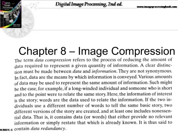
4. Data vs Information • Data and information are not synonymous terms! • Datais the means by which information is conveyed. • Data compression aims to reduce the amount of data required to represent a given quantity of information while preserving as much information as possible.

5. Data vs Information (cont’d) • The same amount of information can be represented by various amount of data, e.g.: Ex1: Your wife, Helen, will meet you at Logan Airport in Boston at 5 minutes past 6:00 pm tomorrow night Your wife will meet you at Logan Airport at 5 minutes past 6:00 pm tomorrow night Helen will meet you at Logan at 6:00 pm tomorrow night Ex2: Ex3:

6. Data Redundancy • Data redundancy is a mathematically quantifiable entity! compression

7. Data Redundancy (cont’d) • Compression ratio: • Relative data redundancy: Example:

8. Types of Data Redundancy (1) Coding redundancy (2) Interpixel redundancy (3) Psychovisual redundancy • The role of compression is to reduce one or more of these redundancy types.

9. Coding Redundancy Data compression can be achieved using an appropriate encoding scheme. Example: binary encoding

10. Encoding Schemes • Elements of an encoding scheme: • Code: a list of symbols (letters, numbers, bits etc.) • Code word: a sequence of symbols used to represent a piece of information or an event (e.g., gray levels) • Code word length: number of symbols in each code word

11. Definitions • In an MxN gray level image • Let be a discrete random variable representing the gray levels in an • image. Its probability is represented by

12. Constant Length Coding • l(rk) = c which implies that Lavg=c Example:

13. Avoiding Coding Redundancy • To avoid coding redundancy, codes should be selected according to the probabilities of the events. • Variable Length Coding • Assign fewer symbols (bits) to the more probable events (e.g., gray levels for images)

14. Variable Length Coding • Consider the probability of the gray levels: variable length

15. Interpixel redundancy • This type of redundancy – sometimes called spatial redundancy, interframe redundancy, or geometric redundancy – exploits the fact that an image very often contains strongly correlated pixels, in other words, large regions whose pixel values are the same or almost the same.

16. Interpixel redundancy • Interpixel redundancy implies that any pixel value can be reasonably predicted by its neighbors (i.e., correlated).

17. Interpixel redundancy • This redundancy can be explored in several ways, one of which is by predicting a pixel value based on the values of its neighboring pixels. • In order to do so, the original 2-D array of pixels is usually mapped into a different format, e.g., an array of differences between adjacent pixels. • If the original image pixels can be reconstructed from the transformed data set the mapping is said to be reversible.

18. Interpixel redundancy (cont’d) • To reduce interpixel redundnacy, the data must be transformed in another format (i.e., through mappings) • e.g., thresholding, or differences between adjacent pixels, or DFT • Example: (profile – line 100) original threshold binary

19. Psychovisual redundancy • Takes into advantage the peculiarities of the human visual system. • The eye does not respond with equal sensitivity to all visual information. • Humans search for important features (e.g., edges, texture, etc.) and do not perform quantitative analysis of every pixel in the image.

20. Psychovisual redundancy (cont’d)Example: Quantization 16 gray levels improved gray-scale quantization 256 gray levels 16 gray levels 8/4 = 2:1 i.e., add to each pixel a pseudo-random number prior to quantization(IGS)

21. Fidelity Criteria How close is to ? Criteria Subjective: based on human observers Objective: mathematically defined criteria

22. Subjective Fidelity Criteria

23. Objective Fidelity Criteria Root mean square error (RMS) Mean-square signal-to-noise ratio (SNR)

24. Example RMS=5.17 RMS=15.67 RMS=14.17 original

25. Image Compression Model

26. Image Compression Model (cont’d) • Mapper: transforms the input data into a format that facilitates reduction of interpixel redundancies.

27. Image Compression Model (cont’d) Quantizer: reduces the accuracy of the mapper’s output in accordance with some pre-established fidelity criteria.

28. Image Compression Model (cont’d) Symbol encoder: assigns the shortest code to the most frequently occurring output values.

29. Image Compression Models (cont’d) • The inverse operations are performed. • But … quantization is irreversible in general.

30. The Channel Encoder and Decoder • As the output of the source encoder contains little redundancy it would be highly sensitive to transmission noise. • • Channel Encoder is used to introduce redundancy in a controlled fashion when the channel is noisy. • Example: Hamming code

31. The Channel Encoder and Decoder It is based upon appending enough bits to the data being encoded to ensure that some minimum number of bits must change between valid code words. The 7-bit hamming (7,4) code word h1…..h7

32. The Channel Encoder and Decoder • Any single bit error can be detected and corrected • any error indicated by non-zero parity word c4,2,1

33. How do we measure information? • What is the information content of a message/image? • What is the minimum amount of data that is sufficient to describe completely an image without loss of information?

34. Modeling the Information Generation Process • Assume that information generation process is a probabilistic process. • A random event E which occurs with probability P(E) contains:

35. How much information does a pixel contain? • Suppose that the gray level value of pixels is generated by a random variable, then rk contains units of information

36. Average information of an image • Entropy: the average information content of an image using we have: units/pixel Assumption:statistically independent random events

37. Modeling the Information Generation Process (cont’d) • Redundancy: where:

38. Entropy Estimation • Not easy! image

39. Entropy Estimation First order estimate of H:

40. Estimating Entropy (cont’d) • Second order estimate of H: • Use relative frequencies of pixel blocks : image

41. Estimating Entropy (cont’d) • Comments on first and second order entropy estimates: • The first-order estimate gives only a lower-bound on the compression that can be achieved. • Differences between higher-order estimates of entropy and the first-order estimate indicate the presence of interpixel redundancies.

42. Estimating Entropy (cont’d) • E.g., consider difference image:

43. Estimating Entropy (cont’d) • Entropy of difference image: • Better than before (i.e., H=1.81 for original image), • however, a better transformation could be found:

44. Lossless Compression • Huffman, Golomb, Arithmetic  coding redundancy • LZW, Run-length, Symbol-based, Bit-plane  interpixel redundancy

45. Huffman Coding (i.e., removes coding redundancy) • It is a variable-length coding technique. • It creates the optimal code for a set of source symbols. • Assumption: symbols are encoded one at a time!

46. Huffman Coding (cont’d) • Optimal code: minimizes the number of code symbols per source symbol. • Forward Pass • 1. Sort probabilities per symbol • 2. Combine the lowest two probabilities • 3. Repeat Step2 until only two probabilities remain.

47. Huffman Coding (cont’d) • Backward Pass Assign code symbols going backwards

48. Huffman Coding (cont’d) • Lavg using Huffman coding: • Lavg assuming binary codes:

49. Huffman Coding (cont’d) • Comments • After the code has been created, coding/decoding can be implemented using a look-up table. • Decoding can be done in an unambiguous way !!

50. Arithmetic (or Range) Coding (i.e., removes coding redundancy) • No assumption on encoding symbols one at a time. • No one-to-one correspondence between source and code words. • Slower than Huffman coding but typically achieves better compression. • A sequence of source symbols is assigned a single arithmetic code word which corresponds to a sub-interval in [0,1]