CH 8. Image Compression
CH 8. Image Compression. 8.1 Fundamental 8.2 Image compression models 8.3 Elements of information theory 8.4 Error-free compression 8.5 Lossy compression 8.6 Image compression standards. 8.1 Fundamentals.


CH 8. Image Compression
E N D
Presentation Transcript
CH 8. Image Compression 8.1 Fundamental 8.2 Image compression models 8.3 Elements of information theory 8.4 Error-free compression 8.5 Lossy compression 8.6 Image compression standards
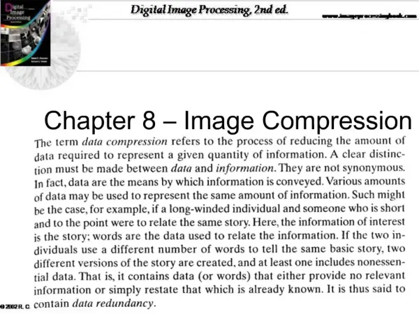
8.1 Fundamentals • Data compression aims to reducethe amount of data while preservingas much information as possible. • The goal of image compression is to reduce the amount of data required to represent an image.
Lossless • Information preserving • Low compression ratios • Lossy • Not information preserving • High compression ratios Trade-off:information loss vs. compression ratio
Compression Ratio compression Compression ratio:
Relevant Data Redundancy Example:
Types of Data Redundancy (1) Coding Redundancy (2) Interpixel Redundancy (3) Psychovisual Redundancy • Data compression attempts to reduce one or more of these redundancy types.
Coding - Definitions Code: a list of symbols (letters, numbers, bits etc.) Code word: a sequence of symbols used to represent some information (e.g., gray levels). Code word length: number of symbols in a code word.
Coding - Definitions (cont’d) N x M image, rk: k-th gray level l(rk):# of bits for rk, P(rk): probability of rk Expected value:
8.1.1 Coding Redundancy • Case 1:l(rk) = constant length Example:
8.1.1 Coding Redundancy (cont’d) • Case 2:l(rk) = variable length variable length Total number of bits: 2.7NM
8.1.2 Interpixel redundancy • Interpixelredundancy implies that pixel values are correlated (i.e., a pixel value can be reasonably predicted by its neighbors). histograms auto-correlation auto-correlation: f(x)=g(x)
8.1.2 Interpixel redundancy • To reduce interpixelredundancy, some kind of transformation must be applied on the data (e.g., thresholding, DFT, DWT) Example: threshold original 11 ……………0000……………………..11…..000….. thresholded (1+10) bits/pair
8.1.3 Psychovisual redundancy • The human eye is more sensitive to the lower frequencies than to the higher frequencies in the visual spectrum. • Idea:discard data that is perceptually insignificant!
8.1.3 Psychovisual redundancy Example: quantization 16 gray levels + random noise 16 gray levels 256 gray levels add a small pseudo-random number to each pixel prior to quantization C=8/4 = 2:1
8.1.4 Fidelity Criteria How close is to ? Criteria Subjective: based on human observers Objective: mathematically defined criteria
Objective Fidelity Criteria Root mean square error (RMS) Mean-square signal-to-noise ratio (SNR)
Image Compression Models (cont’d) • The decoder applies the inverse steps. • Note that quantization is irreversiblein general.
8.3 Element of Info Theory • A key question in image compression is: • How do we measure the information content of an image? “What is the minimum amount of data that is sufficient to describe completely an image without loss of information?”
8.3.1 Measuring Information • We assume that information generation is a probabilistic process. • Idea: associate information with probability! A random event E withprobability P(E) contains: Note: I(E)=0 when P(E)=1
How much information does a pixel contain? • Suppose that gray level values are generated by a random process, then rkcontains: units of information! (assume statistically independent random events)
How much information does a pixel contain? • Average information content of an image: using units/pixel (e.g., bits/pixel) Entropy:
8.3.4 Using Information Theory • Redundancy: where: Note: if Lavg= H, then R=0 (no redundancy)
Entropy Estimation • It is not easy to estimate H reliably! image
Entropy Estimation (cont’d) First order estimate of H: Lavg = 8 bits/pixel R= Lavg-H The first-order estimate provides only a lower-bound on the compression that can be achieved.
Entropy Estimation (cont’d) • Second order estimate of H: • Use relative frequencies of pixel blocks (adjacent pair): image
Differences in Entropy Estimates • Differences between higher-order estimates of entropy and the first-order estimate indicate the presence of interpixelredundancy! • Need to apply some transformationto deal with interpixelredundancy!
Differences in Entropy Estimates (cont’d) • For example, consider pixel differences: 16
Differences in Entropy Estimates (cont’d) • What is the entropy of the difference image? (better than the entropy of the original image H=1.81) • An even better transformation is possible • since the second order entropy estimate is lower: