Download
1 / 65
650 likes | 811 Vues
Learn about image compression theory, techniques, and standards. Explore lossless and lossy compression models, information theory basics, and practical applications like JPEG. Prepare for the final exam with essential concepts and evaluation criteria.

E N D
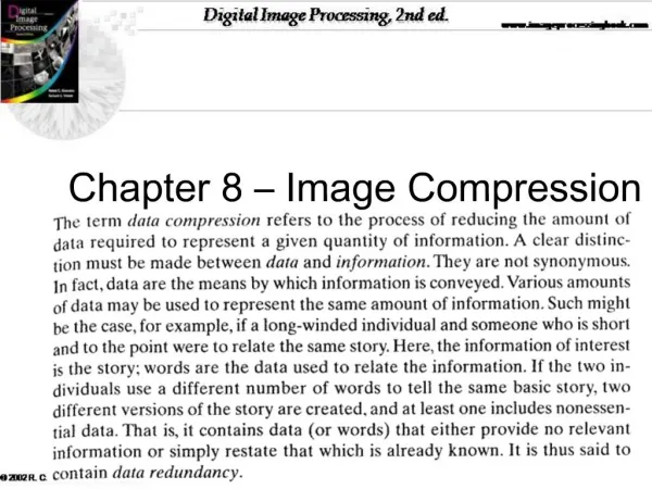
CH 8. Image Compression 8.1 Fundamental 8.2 Image compression model 8.3 Elementary of information theory 8.4 Error-free(Lossless) compression 8.5 Lossy compression-JPEG 8.6 Image compression standards
Final Exam • FinalExam Registration: until 4th July(Mon) • Final Exam Date & Time: 20th July(Wed), 2016 10:00-12:00 • Place: Z613 ( D436) • Evaluation sheet
How is HVS sensitivity? • Lossy encoding Frequency sensitivity of Human Visual System
Lossy Compression • Transform the image into some other domain to reduce interpixelredundancy. ~ (N/n)2 subimages
Example: Fourier Transform Note that the magnitude of the FT decreases, as u, v increase! K << N K-1 K-1
Transform Selection • T(u,v) can be computed using various transformations, for example: • DFT • DCT (Discrete Cosine Transform) • KLT (Karhunen-LoeveTransformation) or Principal Component Analysis (PCA) • JPEG using DCT for handling interpixelredundancy.
DCT (Discrete Cosine Transform) Forward: Inverse: if u=0 if v=0 if v>0 if u>0
DCT (cont’d) • Basis functions for a 4x4 image (i.e., cosines of different frequencies).
DCT (cont’d) DFT WHT DCT Using 8 x 8 sub-images yields 64 coefficients per sub-image. Reconstructed images by truncating 50% of the coefficients More compact transformation RMS error: 2.32 1.78 1.13
DCT (cont’d) • Sub-image size selection: Reconstructions 2 x 2sub-images 4 x 4sub-images 8 x 8sub-images original
DCT (cont’d) • DCT minimizes "blocking artifacts" (i.e., boundaries between subimagesdo not become very visible). DFT has n-point periodicity DCT has 2n-point periodicity
JPEG - Steps 1. Divide image into 8x8 subimages. For each subimage do: 2.Shift the gray-levels in the range [-128, 127] 3.Apply DCT 64 coefficients 1 DC coefficient: F(0,0) 63 AC coefficients: F(u,v)
Example [-128, 127] (non-centered spectrum)
JPEG Steps 4.Quantize the coefficients (i.e., reduce the amplitude of coefficients that do not contribute a lot). Q(u,v): quantization table
Example • Simple Quantization Table Q[i][j]
Example (cont’d) Quantization
JPEG Steps (cont’d) 5.Order the coefficients using zig-zagordering - Creates long runs of zeros (i.e., ideal for run-length encoding)
JPEG Steps (cont’d) 6.Encode coefficients: 6.1 Form “intermediate” symbol sequence. 6.2 Encode “intermediate” symbol sequence into a binary sequence.
Intermediate Symbol Sequence – DC coeff symbol_1 (SIZE)symbol_2 (AMPLITUDE) DC (6) (61) SIZE: # bits need to encode the coefficient
DC Coefficient Encoding symbol_1 symbol_2 (SIZE) (AMPLITUDE) predictive coding:
Intermediate Symbol Sequence – AC coeff symbol_1 (RUN-LENGTH, SIZE)symbol_2 (AMPLITUDE) end of block AC (0, 2) (-3) RUN-LENGTH: run of zeros preceding coefficient SIZE: # bits for encoding the amplitude of coefficient Note: If RUN-LENGTH > 15, use symbol (15,0) ,
Example: AC Coefficients Encoding AC (0,2) (-3) (01 00)
Final Symbol Sequence 1110 111101 01 00 100 0100 ……….
What is the effect of the “Quality” parameter? (8k bytes) (58k bytes) (21k bytes) higher compression lower compression
Effect of Quantization: homogeneous 8 x 8 block (cont’d) Quantized De-quantized
Effect of Quantization: homogeneous 8 x 8 block (cont’d) Reconstructed Error is low! Original
Effect of Quantization: non-homogeneous 8 x 8 block (cont’d) Quantized De-quantized
Effect of Quantization: non-homogeneous 8 x 8 block (cont’d) Reconstructed Error is high! Original:
8.6 Image compression standards • JPEG supports several different modes • Sequential Mode – Baseline • Progressive Mode • Hierarchical Mode • Lossless Mode • The default mode is “sequential” • Image is encoded in a single scan (left-to-right, top-to-bottom).
Progressive JPEG • Image is encoded in multiple scans, in order to produce a quick, rough decoded image when transmission time is long. Sequential Progressive
Progressive JPEG (cont’d) • Each scan encodes a subset of DCT coefficients. • We’ll examine the following algorithms: (1) Progressive spectral selection algorithm (2) Progressive successive approximation algorithm (3) Combined progressive algorithm
Progressive JPEG (cont’d) (1) Progressive spectral selection algorithm • Group DCT coefficients into several spectral bands • Send low-frequency DCT coefficients first • Send higher-frequency DCT coefficients next
Progressive JPEG (cont’d) (2) Progressive successive approximation algorithm • Send all DCT coefficients but with lower precision. • Refine DCT coefficients in later scans.
Example after 0.9s after 1.6s after 3.6s
Progressive JPEG (cont’d) (3) Combined progressive algorithm • Combines spectral selection and successive approximation.
Hierarchical JPEG • Hierarchical mode encodes the image at different resolutions. • Image is transmitted in multiple passes with increased resolution at each pass.