Chapter 8 Image Compression
Chapter 8 Image Compression. Commonly Used Formats:. Portable bit map Family (BMP, Lena 66,616B) Graphics interchange Format (GIF, Lena 70,458B) Tag image file format (TIFF/TIF, Lena 88,508B) JPEG format (JFIF/JFI/JPG, Lena 12,377). Image Data Compression.

Chapter 8 Image Compression
E N D
Presentation Transcript
Commonly Used Formats: • Portable bit map Family (BMP, Lena 66,616B) • Graphics interchange Format (GIF, Lena 70,458B) • Tag image file format (TIFF/TIF, Lena 88,508B) • JPEG format (JFIF/JFI/JPG, Lena 12,377)
Image Data Compression • Large amount of data per image has 3 implications: • storage • processing • communications • For digital image, 512×512×3 bytes/frame = 768Kbyte/frame • Data rate = half of line frequency (e.g. 25Hz), total data rate = 768KB×25/sec = 19.2Mbyte/sec
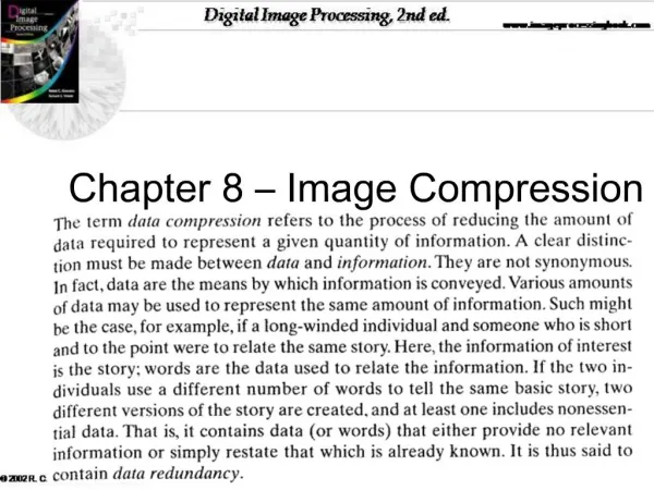
Image Data Compression • The goal of image compression is to reduce the amount of data required to represent a digital image. • Compression can be losslessor lossy. • The strategy is to remove redundant data from the image. • The compressed data should allow the original image to be reconstructed or approximated.
Entropy coding Image Data Compression
Entropy Coding • Consider a source with L possible independent symbols with probabilities pi , i = 0,…,L-1. The entropy is defined as • Shannon’s noise coding theorem: It is possible to code, without distortion, a source of entropy H, using ( ) bits/symbol where can be arbitrarily small.
Ideal compression ratio (without distortion): • Example: If 256 gray level with equal probability, then
i.e. No compression if the gray levels are all random. If are different, then use a variable length code –Huffman coding.
Huffman coding • Arrange the symbol probabilities in a decreasing order and consider them as leaf nodes of a tree. • While there is more than one node: • Merge the 2 nodes with smallest probability. To form a new node, whose probability is the sum of the 2 merged node. • Arbitrarily assign 1 and 0 to each pair of branches merging into a node. • Repeat the above until there is only one symbol left with a probability of 1.
The resultant code is obtained by reading sequentially from the root node to the leaf node where the symbol is located. • Note: There may be a choice between two symbols with the same probability. If this is the case, either symbol can be chosen. The final tree and codes will be different, but the overall efficiency of the code will be the same. • Notice that each string of 0's and 1's can be uniquely decoded. • Coding and decoding – by table lookup.
Encode the letters A (0.12), E (0.42), I (0.09), O (0.30), U (0.07) Thus the codes for each letter are: A - 100 E - 0 I - 1011 O - 11 U - 1010 Now using this code, any string of vowels can be written uniquely. AI = 1001011 EIEIO = 010110101111 UEA = 10100100 10110 = IE 100101011 = AUO 0101111111010 = EIOOU
Run-Length Coding (RLC) • Run‑Coded Binary Images • Run‑coding is an efficient coding scheme for binary or labeled images: not only does it reduce memory space, but it can also speed up image operations. • Example: • Image Row r0000000011111000000000000111000000011111111100000 • Run‑code A • 8(0)5(1)12(0)3(1)7(0)9(1)5(0) • Run‑coding is often used for compression within standard file formats.
Arithmetic Coding • Arithmetic coding is a lossless coding technique. Arithmetic coding typically has a better compression ratio than Huffman coding, as it produces a single symbol rather than several seperate codewords. • a message is represented by an interval of real numbers between 0 and 1. • successive symbols of the message reduce the size of the interval in accordance to the symbols prob. generated by the model.
Start with an interval [0, 1), divided into subintervals of all possible symbols to appear within a message. Make the size of each subinterval proportional to the frequency at which it appears in the message. Eg:
When encoding a symbol, "zoom" into the current interval, and divide it into subintervals like in step one with the new range. Example: suppose we want to encode "addc". We "zoom" into the interval corresponding to "a", and divide up that interval into smaller subintervals like before. We now use this new interval as the basis of the next symbol encoding step.
Repeat the process until the maximum precision of the machine is reached, or all symbols are encoded. To encode the next character “d", we use the "a" interval created before, and zoom into the subinterval “d", and use that for the next step. This produces:
Transmit some number within the latest interval to send the codeword. The number of symbols encoded will be stated in the protocol of the image format, so any number within [0.1804, 0.18432) will be acceptable for “addc”. We last find a shortest binary fraction that lies within [0.1804, 0.18432) to be the codeword. • To decode the message, a similar algorithm is followed, except that the final number is given, and the symbols are decoded sequentially from that.
Bit-plane Encoding • e.g. 256 gray-level image can be considered as 8 one –bit plane • each one-bit plane is coded by RLC • Usually, compression ratio~1.5-2 • Disadvantage: sensitive to noise in transmission.
Predictive Techniques • Remove mutual redundancy between successive pixels and encode only new information. • A quantity , an estimate of u(n) is predicted from the previously decoded samples Whereφdenotes the prediction rule.
Given the prediction rule, we need only to code the error (difference) • And is the quantized value of e(n) • Differential Pulse Code Modulation (DPCM)
Example: • The sequence 100,102,120,120,118,116 is to be predictively coded using the prediction rule for DPCM and a Feedforward predictive coder using . Assume a 2-bit quantizer as shown below:
Giving , we can obtain the following table:
We can see that reconstruction error build up with feedforward system, while error stabilize with DPCM. • Note that if the input sequence is an integer, and the predicted output sequence is made to be an integer, then error=integer and can be coded for perfect reconstruction. • Advantage of quantizer is that the error sequence is distributed over a much smaller range, and hence can be coded with fewer bits.
Delta Modulation (DM) • Simplest form: and a one-bit quanitizer. • Problem: • slope overload [increase sampling rate] • granularity noise [use tri-state DM] • instability to transmission error [use leak, attenuating the predictor output by a factor<1.]
2-D image can be coded line by line. • Each scan line is coded independently by DPCM • Use a 1-D model: • Perform quantization on the error sequence.
2-D DPCM • 2-D prediction model: Where W is a prediction window. • In practice, only nearest neighbour is used.
Transform Coding • Block quantization — a block of data is unitarily transformed so that a large portion of energy is packed in relative few translated coefficients. • It can be shown that the K-L transform is the optional choice — minimize the mean square distortion of the reproduced data for a given no. of bits. • There is no fast algorithm for K-L transform, use DCT usually.
The 2-D DCT of an image f (x,y) is C(u,v), u,v = 0, 1, 2, …, N-1 • By the DCT, image f(x,y) is decomposed into a series expansion of basis functions, which are used as the features
Divide the image into small rectangular (square) blocks • Perform unitary transformation • The coefficients are uniformly quantized but each coefficient with different steps- specified by Quantization Table • The coefficients with more energy is allocated more bits • Entropy encoding- Huffmann coding/Arithmetic Coding (need a code table)
Furthermore, the DC coefficient (the first coefficient in DCT )(which represents the average gray level ) is coded as difference from previous block. • The coefficients are arranged in a zig-zag sequence (in accordance with spatial frequencies)
Subband Coding • To split a multi-dimensional signal into subbands (wavelet decomposition). • Each subband will have different characteristics. • e.g. Human are less sensitive to high freq., hence high freq. Subbands can be coded with fewer bits. • The high freq. subbands will have a smaller range as compared with the original signal.