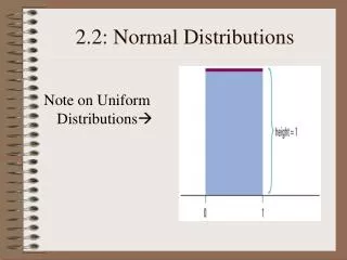
Normal distributions
Normal distributions. The most important continuous probability distribution in the entire filed of statistics is the normal distributions . All normal distributions have the same overall shape.


Normal distributions
E N D
Presentation Transcript
Normal distributions • The most important continuous probability distribution in the entire filed of statistics is the normal distributions. • All normal distributions have the same overall shape. • The exact density curve for a particular normal distribution is specified by giving its mean and its variance 2. • The mean is located at the center of the symmetric density curve and is the same as the median and the mode. • Changing without changing moves the normal curve along the horizontal axis without changing its spread. STA286 week 6
The standard deviation controls the spread of a normal curve. STA286 week 6
The density funstion of the normal random variable is given by • Notation: A normal distribution with mean and variance 2 is denoted by N(, 2). • Note, there are other symmetric bell-shaped density curves that are not normal e.g. t distribution. STA286 week 6
In the normal distribution with mean and standard deviation , Approximately 68% of the observations fall within of the mean . Approximately 95% of the observations fall within 2 of the mean . Approximately 99.7% of the observations fall within 3 of the mean . The 68-95-99.7 rule STA286 week 6
If x is an observation from a distribution that has mean and standard deviation , the standardized value of x is given by A standardized value is often called a z-score. A z-score tells us how many standard deviations the original observation falls away from the mean of the distribution. Standardizing is a linear transformation that transform the data into the standard scale of z-scores. Therefore, standardizing does not change the shape of a distribution, but changes the value of the mean and standard deviation. Standardizing and z-scores STA286 week 6
The heights of women is approximately normal with mean = 64.5 inches and standard deviation = 2.5 inches. The standardized height is The standardized value (z-score) of height 68 inches is or 1.4 std. dev. above the mean. A woman 60 inches tall has standardized height or 1.8 std. dev. below the mean. Example STA286 week 6
The Standard Normal distribution • The standard normal distribution is the normal distribution N(0, 1) that is, the mean = 0 and the sdev = 1 . • If a random variable X has normal distribution N(, ), then the standardized variable has the standard normal distribution. • Areas under a normal curve represent proportion of observations from that normal distribution. • There is no formula to calculate areas under a normal curve. Calculations use either software or a table of areas. The table and most software calculate one kind of area: cumulative proportions . A cumulative proportion is the proportion of observations in a distribution that fall at or below a given value and is also the area under the curve to the left of a given value. STA286 week 6
The standard normal tables • Table A.3 gives cumulative proportions for the standard normal distribution. The table entry for each value z is the area under the curve to the left of z, the notation used is P( Z ≤ z). e.g. P( Z ≤ 1.4 ) = 0.9192 STA286 week 6
Standard Normal Distribution The table shows area to left of ‘z’ under standard normal curve For a negative number, -z : Area below (-z) = Area above (z) = 1 – Area below (z)
The standard normal tables - Example • What proportion of the observations of a N(0,1) distribution takes values a) less than z = 1.4 ? b) greater than z = 1.4 ? c) greater than z = -1.96 ? d) between z = 0.43 and z = 2.15 ? STA286 week 6
Properties of Normal distribution • If a random variable Z has a N(0,1) distribution then P(Z = z)=0. The area under the curve below any point is 0. • The area between any two points a and b (a < b) under the standard normal curve is given by P(a ≤ Z ≤ b) = P(Z ≤ b) – P(Z ≤ a) • As mentioned earlier, if a random variable X has a N(, ) distribution, then the standardized variable has a standard normal distribution and any calculations about X can be done using the following rules: STA286 week 6
P(X = k) = 0 for all k. • The solution to the equation P(X≤ k) = p is k = μ + σzp Where zpis the value z from the standard normal table that has area (and cumulative proportion) p below it, i.e. zp is the pth percentile of the standard normal distribution. STA286 week 6
1. The marks of STA286 students has N(65, 15) distribution. Find the proportion of students having marks (a) less then 50. (b) greater than 80. (c) between 50 and 80. 2. Scores on SAT verbal test follow approximately the N(505, 110) distribution. How high must a student score in order to place in the top 10% of all students taking the SAT? 3. The time it takes to complete a STA286 term test is normally distributed with mean 100 minutes and standard deviation 14 minutes. How much time should be allowed if we wish to ensure that at least 9 out of 10 students (on average) can complete it? Questions STA286 week 6
General Motors of Canada has a deal: ‘an oil filter and lube job in 25 minutes or the next one free’. Suppose that you worked for GM and knew that the time needed to provide these services was approximately normal with mean 15 minutes and std. dev. 2.5 minutes. How many minutes would you have recommended to put in the ad above if it was decided that about 5 free services for 100 customers was reasonable? • In a survey of patients of a rehabilitation hospital the mean length of stay in the hospital was 12 weeks with a std. dev. of 1 week. The distribution was approximately normal. • Out of 100 patients how many would you expect to stay longer than 13 weeks? • What is the percentile rank of a stay of 11.3 weeks? • What percentage of patients would you expect to be in longer than 12 weeks? • What is the length of stay at the 90th percentile? • What is the median length of stay? STA286 week 6
Normal Approximation to the Binomial • If X has a Binomial distribution with mean µ = np and variance σ2 = npq, then the limiting form of the distribution of as n∞, is the standard normal distribution. • It turns out that the normal distribution provides a fairly good approximation even when n is not so large (section 6.5). • As a rule of thumb, we will use this approximation for values of n and p that satisfy np ≥ 10 and n(1-p) ≥ 10 . week 8
Example • You are planning a sample survey of small businesses in your area. You will choose a SRS of businesses listed in the Yellow Pages. Experience shows that only about half the businesses you contact will respond. • If you contact 150 businesses, it is reasonable to use the Bin(150; 0.5) distribution for the number X who respond. Explain why. (b) What is the expected number (the mean) who will respond? (c) What is the probability that 70 or fewer will respond? (d) How large a sample must you take to increase the mean number of respondents to 100? week 8
Exercise • According to government data, 21% of American children under the age of six live in households with incomes less than the official poverty level. A study of learning in early childhood chooses a SRS of 300 children. • What is the mean number of children in the sample who come from poverty-level households? What is the standard deviation of this number? b) Use the normal approximation to calculate the probability that at least 80 of the children in the sample live in poverty. week 8
The Chi-Square distribution • The Chi-Squared densities are subsets of the gamma family of distributions. They are obtained by letting α = υ/2 and λ = ½ where υ is a positive integer. • The parameter of the Chi-Squared distribution, υ, is called degrees of freedom. • The Chi-Squared density is given by • The mean and variance of the Chi-Squared distribution are… week 6
Note: • We can use Table A.5 in Appendix to answer questions like: Find the value k for which . k is the upper 2.5 percentile of the distribution. Notation: . week 6
Weibull Distribution • The continuous random variable X has a Weibull Distribution, with parameters α and β if its density function is given by • The mean and variance of the Weibull Distribution are… • The Weibull distribution is applied to reliability and life-testing problems such as time to failure or life length. • The Weibull distribution does not have the lack of memory property. • The cumulative distribution function is given by… STA286 week 6
Example Service life, in years of an hearing aid battery is a random variable having a Weibull distribution with α = ½ and β = 2. a) How long can such battery be expected to last? b) What is the probability that such a battery will be operating after 2 years? STA286 week 6
Failure Rate for the Weibull Distribution • The time to failure, T, of a component is often described by the Weilbull distribution. • The Weilbull distribution is helpful in determining the failure rate (also called hazard rate) in order to get a sense of wear or deterioration of the component. • The reliability of a component is the probability that it will last for at least a specified time under specific experimental conditions. • The reliability of a component at time t is given by STA286 week 6
The failure rate of a component is the change over time of the conditional probability that the component last an additional ∆t units of time given that it has lasted to time t. • The failure rate at time t is given by: • If β = 1, Z(t) = α which is a constant. This is a special case of the Exponential distribution which has lack of memory. • If β > 1, Z(t) is an increasing function of t indicating that the components wears over time. • If β < 1, Z(t) is a decreasing function of t indicating that the components strengthens over time. STA286 week 6
Example • The live of a certain automobile seal has the Weibull distribution with failure rate given by: • Find the probability that the seal is still intact after 4 year. STA286 week 6