Normal Probability Distributions
Chapter 5. Normal Probability Distributions. Introduction to Normal Distributions and the Standard Distribution. § 5.1. Hours spent studying in a day. 0. 3. 6. 9. 12. 15. 18. 21. 24. The time spent studying can be any number between 0 and 24. Properties of Normal Distributions.


Normal Probability Distributions
E N D
Presentation Transcript
Chapter 5 Normal Probability Distributions
Introduction to Normal Distributions and the Standard Distribution § 5.1
Hours spent studying in a day 0 3 6 9 12 15 18 21 24 The time spent studying can be any number between 0 and 24. Properties of Normal Distributions A continuous random variable has an infinite number of possible values that can be represented by an interval on the number line. The probability distribution of a continuous random variable is called acontinuous probability distribution.
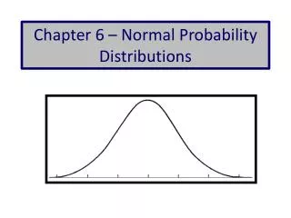
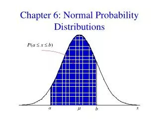
Normal curve x Properties of Normal Distributions The most important probability distribution in statistics is the normaldistribution. A normal distribution is a continuous probability distribution for a random variable, x. The graph of a normal distribution is called the normalcurve.
Properties of Normal Distributions • Properties of a Normal Distribution • The mean, median, and mode are equal. • The normal curve is bell-shaped and symmetric about the mean. • The total area under the curve is equal to one. • The normal curve approaches, but never touches the x-axis as it extends farther and farther away from the mean. • Between μ σ and μ+ σ (in the center of the curve), the graph curves downward. The graph curves upward to the left of μ σ and to the right of μ+ σ. The points at which the curve changes from curving upward to curving downward are called the inflection points.
Inflectionpoints Totalarea= 1 If x is a continuous random variable having a normal distribution with mean μ and standard deviation σ, you can graph a normal curve with the equation Properties of Normal Distributions x μ μ+ σ μ+ 2σ μ+ 3σ μ 3σ μ 2σ μ σ
Inflection points Inflection points x x 1 2 3 4 5 6 7 8 9 10 11 1 2 3 4 5 6 Means and Standard Deviations A normal distribution can have any mean and any positive standard deviation. The mean gives the location of the line of symmetry. Mean:μ = 3.5 Standard deviation: σ 1.3 Mean: μ = 6 Standard deviation: σ 1.9 The standard deviation describes the spread of the data.
B A x 1 3 5 7 9 11 13 Means and Standard Deviations • Example: • Which curve has the greater mean? • Which curve has the greater standard deviation? The line of symmetry of curve A occurs at x = 5. The line of symmetry of curve B occurs at x = 9. Curve B has the greater mean. Curve B is more spread out than curve A, so curve B has the greater standard deviation.
μ = 8 x 6 7 8 9 10 Height (in feet) Interpreting Graphs Example: The heights of fully grown magnolia bushes are normally distributed. The curve represents the distribution. What is the mean height of a fully grown magnolia bush? Estimate the standard deviation. The inflection points are one standard deviation away from the mean. σ 0.7 The heights of the magnolia bushes are normally distributed with a mean height of about 8 feet and a standard deviation of about 0.7 feet.
z 0 1 2 3 3 2 1 The Standard Normal Distribution The standard normal distribution is a normal distribution with a mean of 0 and a standard deviation of 1. The horizontal scale corresponds to z-scores. Any value can be transformed into a z-score by using the formula
z 0 1 2 3 3 2 1 The Standard Normal Distribution If each data value of a normally distributed random variable x is transformed into a z-score, the result will be the standard normal distribution. The area that falls in the interval under the nonstandard normal curve (the x-values) is the same as the area under the standard normal curve (within the corresponding z-boundaries). After the formula is used to transform an x-value into a z-score, the Standard Normal Table in Appendix B is used to find the cumulative area under the curve.
Area is close to 1. z Area is close to 0. 0 1 2 3 3 2 1 z = 3.49 z = 3.49 z = 0 Area is 0.5000. The Standard Normal Table • Properties of the Standard Normal Distribution • The cumulative area is close to 0 for z-scores close to z = 3.49. • The cumulative area increases as the z-scores increase. • The cumulative area for z = 0 is 0.5000. • The cumulative area is close to 1 for z-scores close to z = 3.49
The Standard Normal Table Example: Find the cumulative area that corresponds to a z-score of 2.71. Appendix B: Standard Normal Table Find the area by finding 2.7 in the left hand column, and then moving across the row to the column under 0.01. The area to the left of z = 2.71 is 0.9966.
The Standard Normal Table Example: Find the cumulative area that corresponds to a z-score of 0.25. Appendix B: Standard Normal Table Find the area by finding 0.2 in the left hand column, and then moving across the row to the column under 0.05. The area to the left of z = 0.25 is 0.4013
2. The area to the left of z = 1.23 is 0.8907. z 0 1.23 1. Use the table to find the area for the z-score. Guidelines for Finding Areas • Finding Areas Under the Standard Normal Curve • Sketch the standard normal curve and shade the appropriate area under the curve. • Find the area by following the directions for each case shown. • To find the area to the left of z, find the area that corresponds to z in the Standard Normal Table.
3. Subtract to find the area to the right of z = 1.23: 1 0.8907 = 0.1093. 2. The area to the left of z = 1.23 is 0.8907. z 0 1.23 1. Use the table to find the area for the z-score. Guidelines for Finding Areas • Finding Areas Under the Standard Normal Curve • To find the area to the right of z, use the Standard Normal Table to find the area that corresponds to z. Then subtract the area from 1.
4. Subtract to find the area of the region between the two z-scores: 0.8907 0.2266 = 0.6641. 2. The area to the left of z = 1.23 is 0.8907. 3. The area to the left of z = 0.75 is 0.2266. z 0 1.23 0.75 1. Use the table to find the area for the z-score. Guidelines for Finding Areas • Finding Areas Under the Standard Normal Curve • To find the area between two z-scores, find the area corresponding to each z-score in the Standard Normal Table. Then subtract the smaller area from the larger area.
z 0 2.33 Guidelines for Finding Areas Example: Find the area under the standard normal curve to the left of z = 2.33. Always draw the curve! From the Standard Normal Table, the area is equal to 0.0099.
0.8264 1 0.8264 = 0.1736 z 0 0.94 Guidelines for Finding Areas Example: Find the area under the standard normal curve to the right of z = 0.94. Always draw the curve! From the Standard Normal Table, the area is equal to 0.1736.
0.8577 0.0239 0.8577 0.0239 = 0.8338 z 1.98 0 1.07 Guidelines for Finding Areas Example: Find the area under the standard normal curve between z = 1.98 and z = 1.07. Always draw the curve! From the Standard Normal Table, the area is equal to 0.8338.