Normal Distributions
Normal Distributions. Continuous Distribution. For a discrete distribution, for example Binomial distribution with n=5, and p=0.4, the probability distribution is x 0 1 2 3 4 5 f(x) 0.07776 0.2592 0.3456 0.2304 0.0768 0.01024. P(x). x.

Normal Distributions
E N D
Presentation Transcript
Continuous Distribution • For a discrete distribution, for example Binomial distribution with n=5, and p=0.4, the probability distribution is x 0 1 2 3 4 5 f(x) 0.07776 0.2592 0.3456 0.2304 0.0768 0.01024
P(x) x A probability histogram
How to describe the distribution of a continuous random variable? • For continuous random variable, we also represent probabilities by areas—not by areas of rectangles, but by areas under continuous curves. • For continuous random variables, the place of histograms will be taken by continuous curves. • Imagine a histogram with narrower and narrower classes. Then we can get a curve by joining the top of the rectangles. This continuous curve is called a probability density (or probability distribution).
Continuous distributions • For any x, P(X=x)=0. (For a continuous distribution, the area under a point is 0.) • Can’t use P(X=x) to describe the probability distribution of X • Instead, consider P(a≤X≤b)
Density function • A curve f(x): f(x) ≥ 0 • The area under the curve is 1 • P(a≤X≤b) is the area between a and b
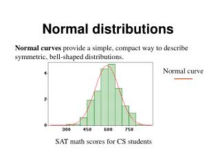
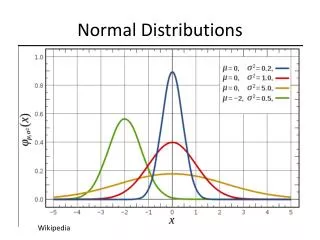
Properties Of Normal Curve • Normal curves are symmetrical. • Normal curves are unimodal. • Normal curves have a bell-shaped form. • Mean, median, and mode all have the same value. • Total area = 1 • Defined by mean and standard deviation (centered at mean)
Percent of Values Within One Standard Deviations 68.26% of Cases
Percent of Values Within Two Standard Deviations 95.44% of Cases
Percent of Values Within Three Standard Deviations 99.72% of Cases
Standard Scores (Z-scores) • Expressed in standard deviations from mean • There are many kinds of Standard Scores. The most common standard score is the ‘z’ scores. • A ‘z’ score states the number of standard deviations by which the original score lies above or below the mean of a normal curve.
Commonly used probabilities and z-scores: Middle 90%: between -1.645 and +1.645 Middle 95%: between -1.96 and +1.96 Middle 99%: between -2.576 and +2.576 90th percentile: 1.28 95th percentile: 1.645 99th percentile: 2.33
Area When Score is Known • For a normal distribution with mean of 100 and standard deviation of 20, what proportion of cases fall below 80? • ~16%
Calculator: Normal cumulative density function: normalcdf(left bound, right bound, mean, st. dev.) (mean and st. dev. default to 0 and 1) To find z-scores given the area in the left tail of a normal distribution: invNorm(area, mean, standard deviation)
Score When Area Is Known • For a normal distribution with mean of 100 and standard deviation of 20, find the score that separates the upper 20% of the cases from the lower 80% • Answer = 116.8
Ways to Assess Normality Use graphs (dotplots, boxplots, or histograms) Normal probability (quantile) plot
Normal Probability (Quartile) plots The observation (x) is plotted against known normal z-scores If the points on the quantile plot lie close to a straight line, then the data is normally distributed Deviations on the quantile plot indicate nonnormal data Points far away from the plot indicate outliers Vertical stacks of points (repeated observations of the same number) is calledgranularity
Are these approximately normally distributed? 50 48 54 47 51 52 46 53 52 51 48 48 54 55 57 45 53 50 47 49 50 56 53 52 What is this called? The normal probability plot is approximately linear, so these data are approximately normal. Both the histogram & boxplot are approximately symmetrical, so these data are approximately normal.


