Normal Distributions
Normal Distributions. Section 4.4. Normal Distribution Function. Among all the possible probability density functions, there is an important class of functions called normal density functions , or normal distributions .


Normal Distributions
E N D
Presentation Transcript
Normal Distributions Section 4.4
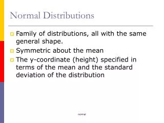
Normal Distribution Function Among all the possible probability density functions, there is an important class of functions called normal density functions, or normal distributions. The graph of a normal density function is bell-shaped andsymmetric, as the following figure shows.
Normal Distribution Function • A normal distribution, is a function of the form • where μ is the mean and σ is the standard deviation.
Graphs of Normal Distributions • The “inflection points” are the points where the curve changes from bending in one direction to bending in another. • Figure below shows the graph of several normal distribution functions. • The third of these has mean 0 and standard deviation 1, and is called the standard normal distribution. • We use Z rather than X to refer to the standard normal variable.
Calculate Probability using Standard Normal Distribution function • The standard normal distribution has μ = 0 and σ = 1. The corresponding variable is called the standard normal variable, which we always denote by Z. • Recall that to calculate the probability P(a ≤ Z ≤ b), we need to find the area under the distribution curve between the vertical lines z = a and z = b. • We can use the table in the Appendix to look up these areas. Here is an example.
Example 1 • Let Z be the standard normal variable. Calculate the following probabilities: • a. P(0 ≤ Z ≤ 2.4) • b. P(0 ≤ Z ≤ 2.43) • c. P(–1.37 ≤ Z ≤ 2.43) • d. P(1.37 ≤ Z ≤ 2.43)
Example 1a • We are asking for the shaded area under the standard normal curve shown in the graph below. • We can find this area, correct to four decimal places, by looking at the table in the Appendix, which lists the area under the standard normal curve from Z = 0 to Z = b for any value of b between 0 and 3.09.
Example 1a continued • To use the table, write 2.4 as 2.40, and read the entry in the row labeled 2.4 and the column labeled .00 (2.4 + .00 = 2.40). Here is the relevant portion of the table: • Thus, P(0 ≤ Z ≤ 2.40) = .4918.
Example 1b • The area we require can be read from the same portion of the table shown above. Write 2.43 as 2.4 + .03, and read the entry in the row labeled 2.4 and the column labeled .03: • Thus, P(0 ≤ Z ≤ 2.43) = .4925.
Example 1c • Here we cannot use the table directly because the range –1.37 ≤ Z ≤ 2.43 does not start at 0. But we can break the area up into two smaller areas that start or end at 0: • P(–1.37 ≤ Z ≤ 2.43) = P(–1.37 ≤ Z ≤ 0) + P(0 ≤ Z ≤ 2.43). • In terms of the graph, we are splitting the desired area into two smaller areas.
Example 1c continued • We already calculated the area of the right-hand piece in part (b): • P(0 ≤ Z ≤ 2.43) = .4925. • For the left-hand piece, the symmetry of the normal curve tells us that • P(–1.37 ≤ Z ≤ 0) = P(0 ≤ Z ≤ 1.37). • This we can find on the table. Look at the row labeled 1.3 and the column labeled .07, and read • P(–1.37 ≤ Z ≤ 0) = P(0 ≤ Z ≤ 1.37) • = .4147. • Thus, • P(–1.37 ≤ Z ≤ 2.43) = P(–1.37 ≤ Z ≤ 0) + P(0 ≤ Z ≤ 2.43) • = .4147 + .4925 • = .9072.
Example 1d • The range 1.37 ≤ Z ≤ 2.43 does not contain 0, so we cannot use the technique of part (c). Instead, the corresponding area can be computed as the difference of two areas: • P(1.37 ≤ Z ≤ 2.43) = P(0 ≤ Z ≤ 2.43) – P(0 ≤ Z ≤ 1.37) • = .4925 – .4147 • = .0778.
Calculating probability of any normal distribution • Although we have tables to compute the area under the standard normal curve, there are no readily available tables for nonstandard distributions. • For example, If μ = 2 and σ = 3, then how would we calculate P(0.5 ≤ X ≤ 3.2)? The following conversion formula provides a method for doing so: • Standardizing a Normal DistributionIf X has a normal distribution with mean μ and standard deviation σ , and if Z is the standard normal variable, then
Quick example • If μ = 2 and σ = 3, then • = P(−0.5 ≤ Z ≤ 0.4) • = .1915 + .1554 • = .3469.
Example 2 • Pressure gauges manufactured by Precision Corp. must be checked for accuracy before being placed on the market. • To test a pressure gauge, a worker uses it to measure thepressure of a sample of compressed air known to be at a pressure of exactly 50 pounds per square inch. If the gauge reading is off by more than 1% (0.5 pounds), it is rejected.Assuming that the reading of a pressure gauge under these circumstances is a normal random variable with mean 50 and standard deviation 0.4, find the percentage of gaugesrejected.
Example 2 solution • If X is the reading of the gauge, then X has a normal distribution with μ = 50 and σ = 0.4. We are asking forP(X < 49.5 or X > 50.5) = 1 – P(49.5 ≤ X ≤ 50.5). • We calculate • = P(–1.25 ≤ Z ≤ 1.25) • = 2 P(0 ≤ Z ≤ 1.25) • = 2(.3944) • = .7888.
Example 2 solution continued • So, P(X < 49.5 or X > 50.5) = 1 – P(49.5 ≤ X ≤ 50.5) • = 1 – .7888 • = .2112. • In other words, about 21% of the gauges will be rejected.
Calculating probability with any normal distribution • In many applications, we need to know the probability thata value of a normal random variable will lie within one standard deviation of the mean, or within two standard deviations, or within some number of standard deviations. • To compute these probabilities, we first notice that, if X has a normal distribution with mean μ and standard deviation σ, then • P(μ – kσ≤ X ≤ μ + kσ) = P(–k ≤ Z ≤ k) • by the standardizing formula.
1, 2 and 3 standard deviations from the mean. • We can compute these probabilities for various values of k using the table in the Appendix, and we obtain the following results. • Probability of a Normal Distribution Being within kStandard Deviations of Its Mean μ – 2σ μμ+ 2σ P(μ – 2σ X μ + 2σ) = P(–2 Z 2) = .9544 μ – σ μμ + σ P(μ – σ X μ + σ) = P(–1 Z 1) = .6826 μ – 3σ μμ + 3σ P(μ – 3σX μ + 3σ) = P(–3 Z 3) = .9974