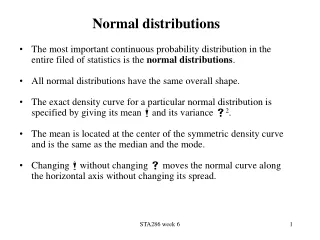
Understanding Normal Distributions: Properties and Applications
This article delves into the concept of normal distributions, illustrated with real-world examples such as the lengths of toilet paper rolls, pig weights, and university student heights. It explains key properties of the normal distribution curve, including the empirical rule, which states that approximately 68%, 95%, and 99.7% of values lie within one, two, and three standard deviations of the mean, respectively. Additionally, practical examples demonstrate how to calculate intervals and z-scores, explaining their significance in determining variability and probabilities in normally distributed data.

Understanding Normal Distributions: Properties and Applications
E N D
Presentation Transcript
Normal Distributions 2013. 10
정규분포의 예 • 두루마리 화장지의 길이 • 돼지 몸무게 • 대학교 4학년 남학생의 키 • 광장동의 집값 • 은행의 이자율 등
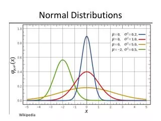
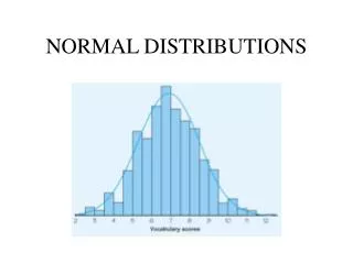
Properties of Normal Distribution Curve • The normal (distribution) curve • From μ–σ to μ+σ: contains about 68% of the measurements (μ: mean, σ: standard deviation) • From μ–2σ to μ+2σ: contains about 95% of it • From μ–3σ to μ+3σ: contains about 99.7% of it
Empirical Rule About 95% of the area lies within 2 standard deviations About 99.7% of the area lies within 3 standard deviations of the mean About 68% of the area lies within 1 standard deviation of the mean 68%
Determining Intervals x 3.3 3.6 3.9 4.2 4.5 4.8 5.1 An instruction manual claims that the assembly time for a product is normally distributed with a mean of 4.2 hours and standard deviation 0.3 hour. Determine the interval in which 95% of the assembly times fall. 95% of the data will fall within 2 standard deviations of the mean. 4.2 – 2 (0.3) = 3.6 and 4.2 + 2 (0.3) = 4.8. 95% of the assembly times will be between 3.6 and 4.8 hrs.
The Standard Score The standard score, or z-score, represents the number of standard deviations a random variable x falls from the mean. The test scores for a civil service exam are normally distributed with a mean of 152 and a standard deviation of 7. Find the standard z-score for a person with a score of: (a) 161 (b) 148 (c) 152 (a) (b) (c)
The Standard Normal Distribution The standard normal distribution has a mean of 0 and a standard deviation of 1. Using z-scores any normal distribution can be transformed into the standard normal distribution. z –4 –3 –2 –1 0 1 2 3 4
Cumulative Areas The total area under the curve is one. z –3 –2 –1 0 1 2 3 • The cumulative area is close to 0 for z-scores close to –3.49. • The cumulative area for z = 0 is 0.5000. • The cumulative area is close to 1 for z-scores close to 3.49.
A Practical Exampleof Normal Dist. • Your company packages sugar in 1 kg bags. • When you weigh a sample of bags you get these results: • 1007g, 1032g, 1002g, 983g, 1004g, ... (a hundred measurements) • Mean = 1010g • Standard Deviation = 20g • Some values are less than 1000g ... can you fix that?
The normal distribution of your measurements looks like this: • 31% of the bags are less than 1000g, which is cheating the customer!
How to reduce “less than 1000g sugar bag” ? • if 1000g was at -3 standard deviations there would be only 0.1% (very small) • if 1000g was at -2.5 standard deviations there would be only 0.6% (small) • How ? • increase the amount of sugar in each bag (this would change the mean), or • make it more accurate (this would reduce the standard deviation)
Solution • First method: adjust the mean amount in each bag • 2.5(standard deviation) * 20g = 50g • Second method: Adjust the accuracy of the machine • we can keep the same mean (of 1010g), but then we need 2.5 standard deviations to be equal to 10g: • 10g / 2.5 = 4g, so the standard deviation should be 4g


