Mastering Mathematical Induction: Principles and Examples
This chapter explores mathematical induction, well-ordering principles, and recursive definitions, covering fundamental concepts and providing examples to enhance understanding. Learn how to apply strong induction, recursive algorithms, and ensure program correctness through detailed explanations and illustrative examples. Discover how to reason through mathematical proofs and tackle challenging problems using well-structured induction techniques. Enhance your mathematical skills and problem-solving abilities with this comprehensive guide.

Mastering Mathematical Induction: Principles and Examples
E N D
Presentation Transcript
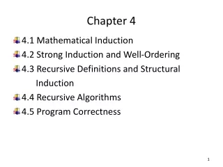
Chapter 4 • 4.1 Mathematical Induction • 4.2 Strong Induction and Well-Ordering • 4.3 Recursive Definitions and Structural Induction • 4.4 Recursive Algorithms • 4.5 Program Correctness
4.1 Induction • A very special rule of inference! • Definition: A set S is well ordered if every subset has a least element. • Note: [0, 1] is not well ordered since (0,1] does not have a least element. • Examples: N is well ordered (under the ≤ relation) • The set of finite strings over an alphabet using lexicographic ordering is well ordered.
4.1 Induction Let P(x) be a predicate over a well ordered set S. • The problem is to prove the rule of inference called The (first) principle of Mathematical induction • In the case that S=N, the nature numbers, the principle has the following form.
4.1 Induction The hypotheses are H1: P(0) ,and H2: P(n)→ P(n+1) for n arbitrary. • H1 is called The Basis Step. • H2 is called The Induction (Inductive) Step. • We first prove that the predicate is true for the smallest element of the set S (0 if S=N) • We then show if it is true for an element x (n if S=N) implies it is true for the “next” element in the set (n+1 if S=N) .
4.1 Induction Then • Knowing it is true for the first element means it must be true for the element following the first or the second element • Knowing it is true for the second element implies it is true for the third, and so forth. Therefore, induction is equivalent to modus ponens applied an countable number of times!!
FIGURE 1 Climbing and Infinite Ladder.
4.1 Induction • We can use the Principle to prove more general assertions because N is well ordered. • Suppose we wish to prove for some specific integer k • Now we merely change the basis step to P(k) and continue. • Example: (a classic) To prove • Example 10: Use mathematical induction to prove the following generalization of one of De Morgan’s Laws: whenever A1, A2,..,An are subsets of a universal set U and n ≥ 2.
4.1 Induction • Example 13: Let n be a positive integer. Show that every 2nX2n checkerboard with one square removed can be tiled using right triominoes, where these pieces cover three squares at a time, as shown below.
4.2 Strong Induction and Well-Ordering • Strong Induction To prove that P(n) is true for all positive integers n, where P(n) is a propositional function, we complete two steps: • Basis Step: We verify that the proposition P(1) is true. • Inductive Step: We show that the conditional statement is true for a all positive integers k. • Example 2: show that if n is an integer greater than 1, then n can be written as the product of primes.
Example 3: consider a game in which two players take turns removing any positive number of matches they want from one of two piles of matches. The player who removes the last match wins the game. Show that if the two piles contain the same number of matches initially, the second player can always guarantee a win. • Example 4: Prove that every amount of postage of 12 cents or more can be formed using just 4-cent and 5-cent stamps.
4.3 Recursive Definitions and Structural Induction • Sometimes it is difficult to define an object explicitly. However, it may be easy to define this object in terms of itself.This process is called recursion. FIGURE 1 A Recursively Defined Picture.
Recursively Defined Functions We use two steps to define a function with the set of nonnegative integers as its domain: • Basis step: specify the value of the function at zero. • Recursive step: give a rule for finding its value at an integer from its values at smaller integers. • Such a definition is called a recursive or inductive definition. • Example 1: suppose that f is defined recursively by f(0)=3, f(n+1)=2*f(n) +3. find f(1) , f(2), f(3), f(4).
Recursively Defined Functions • Example 2: give an inductive definition of the factorial function F(n)=n! . • Example 3: Give a recursive definition of an, where a is a nonzero real number and n is a nonnegative integer. • Example 4: Give a recursive definition of
Recursively Defined Functions • Definition 1: The Fibonacci numbers, f0, f1,f2 ,. . ., are defined by the equations f0=0, f1=1, and fn = fn-1 + fn-2 for n = 2, 3, 4,. . . • Example 5: Find the Fibonacci numbers f2, f3, f4, f5, and f6. • Example 6: Show that whenever n ≥ 3, fn > αn-2, where
Recursively Defined Sets and Structures • Example 7: consider the subset S of the set of integers defined by • Basis step: 3 S. • Recursive step: if x S, y S, then x+y S.
Recursively Defined Sets and Structures • Definition 2: The set * of strings over the alphabet can be defined recursively by • Basis step: *(where λ is the empty string containing no symbols) • Recursive step: if w* and x, then wx* • Example 8: if ={0, 1}, the strings found to be in *, the set of all bit strings, are • λ specified to be in the basis step, • 0 and 1 formed during the first application of the recursive step, • 00, 01, 10, and 11 formed during the second application for the recursive step, and so on.
Recursively Defined Sets and Structures • Definition 3: two strings can be combined via the operation of concatenation. • Let be a set of symbols and • * the set of strings formed form symbols in . • We can define the concatenation of two strings, denoted by ∙ , recursively as follows. • Basis step: if w*, then w ∙λ=w, where λ is the empty string. • Recursive step: if w1* and w2* and x, then w1 ∙(w2x)=(w1 ∙ w2)x • Example 9: length of a string Give a recursive definition of l(w), the length of the string w.
Recursively Defined Sets and Structures • Definition 4: The set of rooted trees, where a rooted tree consists of a set of vertices containing a distinguished vertex called the root, and edges connecting these vertices, can be defined recursively by these steps: • Basis step: A single vertex r is a rooted tree. • Recursive step: Suppose that T1, T2, . . . ,Tnare disjoint rooted trees with roots r1, r2, . . ., rn, respectively. • Then the graph formed by staring with a root r, which is not in any of the rooted trees T1, T2, . . . ,Tn, and adding an edge from r to each of the vertices r1, r2, . . ., rn, is also a rooted tree.
Recursively Defined Sets and Structures FIGURE 2 Building Up Rooted Trees.
Recursively Defined Sets and Structures • Definition 5: The set of extended binary trees can be defined recursively by these step: • Basis step: The empty set is an extended binary tree. • Recursive step: if T1 and T2 are disjoint extended binary trees, there is an extended binary tree, denoted by T1 ∙ T2, consisting of a root r together with edges connecting the root to each of the roots of the left subtree T1and the right subtree T2 when these trees are nonempty.
Recursively Defined Sets and Structures FIGURE 3 Building Up Extended Binary Trees.
Recursively Defined Sets and Structures • Definition 6: The set of full binary trees can be defined recursively by these steps: • Basis step: There is a full binary tree consisting only of a single vertex r. • Recursive step: if T1 and T2are disjoint full binary trees, there is a full binary tree, denoted by T1 ∙ T2, consisting of a root r together with edges connecting the root to each of the roots of the left subtree T1and the right subtree T2 .
Recursively Defined Sets and Structures FIGURE 4 Building Up Full Binary Trees.
Structural Induction • To prove results about recursively defined sets we generally use some form of mathematical induction. • Example 12: show that the set S defined in example 7 by specifying that 3 S and that if x S and y S , then x+y S, is the set of all positive integers that are multiples of 3.
Structural Induction • Definition 7: We define the height h(T) of a full binary tree T recursively. • Basis step: The height of the full binary tree T consisting of only a root r is h(T)=0 • Recursive step: If T1and T2 are full binary trees, then the full binary tree T= T1 ∙T2 has height h(T) = 1+ max(h(T1) , h(T2 )), n(T)+1+n(T1)+n(T2). • Theorem 2: If T is a full binary tree T, then n(T) ≤ 2h(T) +1 -1 Where n(T) is the number of vertex in a full binary tree.
Generalized Induction • As an example, note that we can define an ordering on N x N, the ordered pairs of nonnegative integers, by specifying that (x1, y1) is less than or equal to (x2, y2) if either x1< x2, or x1=x2 and y1 < y2; this is called the lexicographic ordering. • The set N x N with this ordering has the property that every subset of N x N has a least element (see Supplementary exercise 53 in section 8.6). This implies that we can recursively define the terms am,n , with mN, nN, and prove results about them using a variant of mathematical induction, as illustrated in example 15.
Generalized Induction • Example 15: Suppose that am,n is defined recursively for (m, n) N x N by a0,0 =0 and Show that am,n =m+n(n+1)/2 for all (m, n) NxN that is, for all pairs of nonnegative integers.
4.4 Recursive Algorithms • A recursive algorithm is one which calls itself to solve “smaller” versions of an input problem. • How it works: • The current status of the algorithm is placed on a stack. • A stackis a data structure from which entries can be added and deleted only from one end.
like the plates in a cafeteria: • PUSH: put a 'plate' on the stack. • POP: take a 'plate' off the stack. • When an algorithm calls itself, the current activation is suspended in time and its parameters are PUSHed on a stack. • The set of parameters need to restore the algorithm to its current activation is called an activation record.
Example: procedure factorial (n) /* make the procedure idiot proof */ if n < 0 return 'error' if n = 0 then return 1 else return n factorial (n-1) • Algorithm 1A Recursive Algorithm for Computing n! procedurefactorial (n: nonnegative integers) if n=0 thenfactorial(n) :=1 elsefactorial(n) := n.factorial(n-1)
The operating system supplies all the necessary facilities to produce: factorial (3): PUSH 3 on stack and call factorial (2): PUSH 2 on stack and call factorial (1): PUSH 1 on stack and call factorial (0): return 1 POP 1 from stack and return (1) (1) POP 2 from the stack and return (2) [(1) (1)] POP 3 from the stack and return (3) [(2) [(1) (1)]] • Complexity: • Let f(n) be the number of multiplications required to compute factorial (n). f(0) = 0: the initial condition f(n) = 1 + f(n-1): the recurrence equation
Hw :example 2 (p.312) Give a recursive algorithm for computing an, where a is a nonzero real number and n is a nonnegative integer. • Example: • A recursive procedure to find the max of a nonvoid list. • Assume we have a built-in functions called • Length which returns the number of elements in a list • Max which returns the larger of two values • Listhead which returns the first element in a list • Max requires one comparison.
procedure maxlist (list) /* strip off head of list and pass the remainder */ if Length(list) = 1 then return Listhead(list) else return Max( Listhead(list), maxlist (remainder of list)) • The recurrence equation for the number of comparisons required for a list of length n, f(n), is f(1) = 0 f(n) = 1 + f(n-1)
Example: If we assume the length is a power of 2: • We divide the list in half and find the maximum of each half. • Then find the Max of the maximum of the two halves. procedure maxlist2 (list) /* a divide and conquer approach */ if Length (list) = 1 then return Listhead(list) else a = maxlist (fist half of list) b = maxlist (second half of list) return Max{a, b}
Recurrence equation for the number of comparisons required for a list of length n, f(n), is f(1) = 0 f(n) = 2 f(n/2) + 1 • There are two calls to maxlist each of which requires f(n/2) operations to find the max. • There is one comparison required by the Max function.
Algorithm 7A Recursive Algorithm for Fibonacc Numbers. procedurefibonacci (n: nonnegative integers) if n=0 thenfibonacci(0) :=0 else if n=1 thenfibonacci(1) :=1 elsefibonacci(n) := fibonacci(n-1) + fibonacci(n-2) Algorithm 8An Iterative Algorithm for Computing Fibonacci Numbers. procedureiterative fibonacci (n: nonnegative integers) if n=0 theny :=0 else begin x :=0 y :=1 for i :=2 to n begin z :=x+y x :=y y :=z end End {z is the nth Fibonacci number} Recursion and Iteration
The Merge Sort • Example 9: Sort the list 8, 2, 4, 6, 9, 7, 10, 1, 5, 3 using the merge sort. • Algorithm 9A Recursive Merge Sort. Procedure mergesort(L= a1, . . . , an) If n> 1 then Begin m :=n/2 L1 := a1, a2, . . . ,am L2 := am+1, am+2, . . ., an L := merge(mergesort(L1), mergesort(L2)) End {L is now sorted into elements in nondecreasing order}
4.5 Program Correctness • Definition 1: A program, or program segment, S is said to be partially correct with respect tothe initial assertion p and the final assertion q if whenever p is true for the input values of S and S terminates, then q is true for the output values of S. • The notation p{S}q indicates that the program , or program segment, S is partially correct with respect to the initial assertion p and the final assertion q.
Program Verification • Example 1: show that the program segment y := 2 z := x+y is correct with respect to the initial assertion p :x=1 and the final assertion q :z=3.
Rules of Inference • Suppose that the program S is split into subprograms S1 and S2. Write S=S1; S2 to indicate that S is made up of S1 followed by S2. • Suppose that the correctness of S1 with respect to the initial assertion p and final assertion q, and the correctness of S2 with respect to the initial assertion q and the final assertion r, have been established. • It follows that if p is true and S1 is executed and terminates, then q is true; and if q is true, and S2 executes and terminates, then r is true. • This rule of inference, called the composition rule, can be stated as p{S1}q q{S2}r ∴ p{S1 ;S2}r
Conditional Statements Ifcondition then S ,where S is a block of statements. • First , it must be shown that when p is true and condition is also true, then q is true after S terminates. • Example 2: Verify that the program segment if x > y then y := x is correct with respect to the initial assertion T and the final assertion yx.
Conditional Statements • Suppose that a program has a statement of the form If condition then S1 else S2 (pcondition){S1}q (pcondition){S2}q p{if condition then S1 else S2}q • Example 3: verify that the program segment If x < 0 then abs := -x else abs := x is correct with respect to the initial assertion T and the final assertion abs =|x|.
Loop Invariants While condition S • S is repeatedly executed until condition untel condition becomes false. • An assertion that remains true each time S is executed must be chosen. • Such an assertion is called a loop invariant. • In other words, p is a loop invariant if (pcondition){S}p is true. (pcondition){S}p p{while condition S}(conditionp)
Loop Invariants • Example 4: A loop invariant is needed to verify that the program segment i:=1 factorial :=1 while i < n begin i :=i+1 factorial := factorial.i end Terminates with factorial = n! where n is a positive integer.
Example 5: we will outline how to verify the correctness of the program S for computing the product of two integers. The goal is to prove that after S is executed, product has the value mn. Procedure multiply(m,n : integers)

