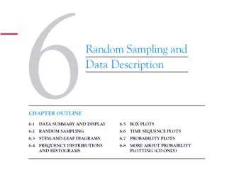
2-1 Data Summary and Display
2-1 Data Summary and Display. Engineering Example
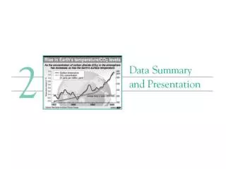

2-1 Data Summary and Display
E N D
Presentation Transcript
Engineering Example Suppose that an engineer is developing a rubber compound for use in O-rings. The O-rings are to be employed as seals in plasma etching tools used in the semiconductor industry, so their resistance to acids and other corrosive substances is an important characteristic. The engineer uses the standard rubber compound to produce eight O-rings in a development laboratory and measures the tensile strength of each specimen after immersion in a nitric acid solution at 30°C for 25 minutes [refer to the American Society for Testing and Materials (ASTM) Standard D 1414 and the associated standards for many interesting aspects of testing rubber O-rings]. The tensile strengths (in psi) of the eight O-rings are 1030, 1035, 1020, 1049, 1028, 1026, 1019, and 1010. Then, he decides to consider a modified formulation of the rubber in which a Teflon additive is included. Eight O-ring specimens are made from this modified rubber compound and subjected to the nitric acid emersion test described earlier. The tensile test results are 1037, 1047, 1066, 1048, 1059, 1073, 1070, and 1040.
2-1 Data Summary and Display Population Mean For a finite population with N measurements, the mean is The sample mean is a reasonable estimate of the population mean.
2-1 Data Summary and Display Sample Variance and Sample Standard Deviation
2-1 Data Summary and Display The sample variance is The sample standard deviation is
2-1 Data Summary and Display Computational formula for s2
2-1 Data Summary and Display Population Variance When the population is finite and consists of N values, we may define the population variance as The sample variance is a reasonable estimate of the population variance.
2-2 Stem-and-Leaf Diagram Steps for Constructing a Stem-and-Leaf Diagram
2-2 Stem-and-Leaf Diagram Percentiles, quartiles, and the median range Median = (40th + 41st )/2=(160+163)/2=161.5 Q1 = (n+1)/4=20.25 btn 20th & 21st Q1= (143+145)/2 = 144 Q2 = median Q3 = 3(n+1)/4 = 60.75 Q3 = (181+181)/2 = 181 IQR = interquartile range = Q3-Q1
2-3 Histograms A histogramis a more compact summary of data than a stem-and-leaf diagram. To construct a histogram for continuous data, we must divide the range of the data into intervals, which are usually called class intervals, cells, or bins. If possible, the bins should be of equal width to enhance the visual information in the histogram.
2-3 Histograms An important variation of the histogram is the Pareto chart. This chart is widely used in quality and process improvement studies where the data usually represent different types of defects, failure modes, or other categories of interest to the analyst. The categories are ordered so that the category with the largest number of frequencies is on the left, followed by the category with the second largest number of frequencies, and so forth.
2-4 Box Plots • The box plotis a graphical display that simultaneously describes several important features of a data set, such as center, spread, departure from symmetry, and identification of observations that lie unusually far from the bulk of the data. • Whisker • Outlier • Extreme outlier
2-4 Box Plots 2nd quartile = median = 161.5 1st quartile = 143.5 3rd quartile = 181 IQR = Q3 – Q1 = 181 – 143.5 = 37.5 1.5 IQR = 56.25 Q3 + 1.5 IQR = 237.25 IQR = Q3 – Q1 = 181 – 143.5 = 37.5 1.5 IQR = 56.25 Q1 - 1.5 IQR = 143.5 – 56.25 = 87.25
SAS code and output OPTIONS NODATE NOOVP NONUMBER; DATA STRENGTH; INPUT STRENGTH @@; CARDS; 105 221 183 186 121 181 180 143 97 154 153 174 120 168 167 141 245 228 174 199 181 158 176 110 163 131 154 115 160 208 158 133 207 180 190 193 194 133 156 123 134 178 76 167 184 135 229 146 218 157 101 171 165 172 158 169 199 151 142 163 145 171 148 158 160 175 149 87 160 237 150 135 196 201 200 176 150 170 118 149 PROCUNIVARIATE DATA=STRENGTH PLOT NORMAL FREQ; VAR STRENGTH; histogram strength/vscale=count; TITLE 'DESCRIPTIVE STATISTICS AND GRAPHS'; /* PROC CHART DATA=STRENGTH; VBAR STRENGTH; VBAR STRENGTH/TYPE=PCT; HBAR STRENGTH/TYPE=CPCT DISCRETE; TITLE 'HISTOGRAM'; */ RUN; QUIT;
DESCRIPTIVE STATISTICS AND GRAPHS UNIVARIATE 프로시저 변수: STRENGTH 적률 N 80 가중합 80 평균 162.6625 관측치 합 13013 표준 편차 33.7732363 분산 1140.63149 왜도 -0.0250253 첨도 0.24027117 제곱합 2206837 수정 제곱합 90109.8875 변동계수 20.7627672 평균의 표준 오차 3.7759626 기본 통계 측도 위치측도 변이측도 평균 162.6625 표준 편차 33.77324 중위수 161.5000 분산 1141 최빈값 158.0000 범위 169.00000 사분위 범위 37.00000 위치모수 검정: Mu0=0 검정 --통계량--- -------p 값------- 스튜던트의 t t 43.07842 Pr > |t| <.0001 부호 M 40 Pr >= |M| <.0001 부호 순위 S 1620 Pr >= |S| <.0001 정규성 검정 검정 ----통계량---- -------p 값------- Shapiro-Wilk W 0.991699 Pr < W 0.8911 Kolmogorov-Smirnov D 0.057091 Pr > D >0.1500 Cramer-von Mises W-Sq 0.046374 Pr > W-Sq >0.2500 Anderson-Darling A-Sq 0.270335 Pr > A-Sq >0.2500 분위수(정의 5) 분위수 추정값 100% 최댓값 245.0 99% 245.0 95% 224.5 90% 204.0 75% Q3 181.0 50% 중위수 161.5 25% Q1 144.0 10% 119.0 5% 103.0 1% 76.0 0% 최솟값 76.0
SAS code and output DESCRIPTIVE STATISTICS AND GRAPHS UNIVARIATE 프로시저 변수: STRENGTH 극 관측치 -----최소---- -----최대---- 값 관측치 값 관측치 76 43 221 2 87 68 228 18 97 9 229 47 101 51 237 70 105 1 245 17 빈도 수 백분율 백분율 백분율 값 빈도 셀 누적 값 빈도 셀 누적 값 빈도 셀 누적 76 1 1.3 1.3 149 2 2.5 31.3 180 2 2.5 73.8 87 1 1.3 2.5 150 2 2.5 33.8 181 2 2.5 76.3 97 1 1.3 3.8 151 1 1.3 35.0 183 1 1.3 77.5 101 1 1.3 5.0 153 1 1.3 36.3 184 1 1.3 78.8 105 1 1.3 6.3 154 2 2.5 38.8 186 1 1.3 80.0 110 1 1.3 7.5 156 1 1.3 40.0 190 1 1.3 81.3 115 1 1.3 8.8 157 1 1.3 41.3 193 1 1.3 82.5 118 1 1.3 10.0 158 4 5.0 46.3 194 1 1.3 83.8 120 1 1.3 11.3 160 3 3.8 50.0 196 1 1.3 85.0 121 1 1.3 12.5 163 2 2.5 52.5 199 2 2.5 87.5 123 1 1.3 13.8 165 1 1.3 53.8 200 1 1.3 88.8 131 1 1.3 15.0 167 2 2.5 56.3 201 1 1.3 90.0 133 2 2.5 17.5 168 1 1.3 57.5 207 1 1.3 91.3 134 1 1.3 18.8 169 1 1.3 58.8 208 1 1.3 92.5 135 2 2.5 21.3 170 1 1.3 60.0 218 1 1.3 93.8 141 1 1.3 22.5 171 2 2.5 62.5 221 1 1.3 95.0 142 1 1.3 23.8 172 1 1.3 63.8 228 1 1.3 96.3 143 1 1.3 25.0 174 2 2.5 66.3 229 1 1.3 97.5 145 1 1.3 26.3 175 1 1.3 67.5 237 1 1.3 98.8 146 1 1.3 27.5 176 2 2.5 70.0 245 1 1.3 100.0 148 1 1.3 28.8 178 1 1.3 71.3
SAS code and output DESCRIPTIVE STATISTICS AND GRAPHS UNIVARIATE 프로시저 변수: STRENGTH 줄기 잎 # 상자그림 24 5 1 0 23 7 1 0 22 189 3 | 21 8 1 | 20 0178 4 | 19 034699 6 | 18 0011346 7 +-----+ 17 0112445668 10 | | 16 0003357789 10 *--+--* 15 001344678888 12 | | 14 12356899 8 +-----+ 13 133455 6 | 12 013 3 | 11 058 3 | 10 15 2 | 9 7 1 | 8 7 1 0 7 6 1 0 ----+----+----+----+ 값: (줄기.잎)*10**+1 정규 확률도 245+ +*+ | *++ | ***+ | *+ | *** | *** | *** | **** | **** | ***** | ****+ | ****+ | **+ | *** | +** | +++* | +++ * 75++* +----+----+----+----+----+----+----+----+----+----+ -2 -1 0 +1 +2
2-5 Time Series Plots • A time seriesor time sequenceis a data set in which the observations are recorded in the order in which they occur. • A time series plotis a graph in which the vertical axis denotes the observed value of the variable (say x) and the horizontal axis denotes the time (which could be minutes, days, years, etc.). • When measurements are plotted as a time series, we often see • trends, • cycles, or • other broad features of the data
SAS code and output OPTIONS NODATE NOOVP NONUMBER LS=80; DATA STRENGTH; INPUT STRENGTH @@; CARDS; 105 221 183 186 121 181 180 143 97 154 153 174 120 168 167 141 245 228 174 199 181 158 176 110 163 131 154 115 160 208 158 133 207 180 190 193 194 133 156 123 134 178 76 167 184 135 229 146 218 157 101 171 165 172 158 169 199 151 142 163 145 171 148 158 160 175 149 87 160 237 150 135 196 201 200 176 150 170 118 149 SYMBOL INTERPOL=JOIN VALUE=DOT HEIGHT=1 LINE=1; PROCGPLOT DATA=STRENGTH; PLOT STRENGTH*N; TITLE 'TIME SERIES GRAPH FOR STRENGTH'; RUN; QUIT;
2-6 Multivariate Data • The dot diagram, stem-and-leaf diagram, histogram, and box plot are descriptive displays for univariate data; that is, they convey descriptive information about a single variable. • Many engineering problems involve collecting and analyzing multivariate data, or data on several different variables. • In engineering studies involving multivariate data, often the objective is to determine the relationships among the variables or to build an empirical model.
2-6 Multivariate Data Sample Correlation Coefficient The strength of a linear relationship between two variables
2-6 Multivariate Data Strong when 0.8≤ r ≤ 1, weak 0 ≤ r ≤ 0.5, and moderate otherwise
SAS code and output OPTIONS NODATE NOOVP NONUMBER LS=80; DATA SHAMPOO; INPUT FOAM SCENT COLOR RESIDUE REGION QUALITY; CARDS; 6.3 5.3 4.8 3.1 1 91 4.4 4.9 3.5 3.9 1 87 3.9 5.3 4.8 4.7 1 82 5.1 4.2 3.1 3.6 1 83 5.6 5.1 5.5 5.1 1 83 4.6 4.7 5.1 4.1 1 84 4.8 4.8 4.8 3.3 1 90 6.5 4.5 4.3 5.2 1 84 8.7 4.3 3.9 2.9 1 97 8.3 3.9 4.7 3.9 1 93 5.1 4.3 4.5 3.6 1 82 3.3 5.4 4.3 3.6 1 84 5.9 5.7 7.2 4.1 2 87 7.7 6.6 6.7 5.6 2 80 7.1 4.4 5.8 4.1 2 84 5.5 5.6 5.6 4.4 2 84 6.3 5.4 4.8 4.6 2 82 4.3 5.5 5.5 4.1 2 79 4.6 4.1 4.3 3.1 2 81 3.4 5 3.4 3.4 2 83 6.4 5.4 6.6 4.8 2 81 5.5 5.3 5.3 3.8 2 84 4.7 4.1 5 3.7 2 83 4.1 4 4.1 4 2 80 PROCCORR DATA=SHAMPOO; VAR FOAM SCENT COLOR RESIDUE REGION QUALITY; TITLE 'CORRELATIONS OF VARIABLES'; PROCSGSCATTER DATA=SHAMPOO; MATRIX FOAM SCENT COLOR RESIDUE REGION QUALITY; TITLE 'MATRIX OF SCATTER PLOTS FOR THE SHAMPOO DATA'; PROCPLOT DATA=SHAMPOO; PLOT QUALITY*FOAM=REGION; TITLE 'SCATTER PLOT OF SHAMPOO QUALITY VS. FORM'; RUN; QUIT: