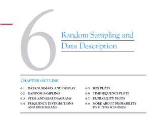
6-1 Data Summary and Display
6-1 Data Summary and Display. Definition. 6-1 Data Summary and Display. Example 6-1. 6-1 Data Summary and Display. Figure 6-1 The sample mean as a balance point for a system of weights. 6-1 Data Summary and Display. Population Mean For a finite population with N measurements, the mean is.

6-1 Data Summary and Display
E N D
Presentation Transcript
6-1 Data Summary and Display Definition
6-1 Data Summary and Display Example 6-1
6-1 Data Summary and Display Figure 6-1The sample mean as a balance point for a system of weights.
6-1 Data Summary and Display Population Mean For a finite population with N measurements, the mean is The sample mean is a reasonable estimate of the population mean.
6-1 Data Summary and Display Definition
6-1 Data Summary and Display How Does the Sample Variance Measure Variability? Figure 6-2How the sample variance measures variability through the deviations .
6-1 Data Summary and Display Example 6-2
6-1 Data Summary and Display Computation of s2
6-1 Data Summary and Display Population Variance When the population is finite and consists of N values, we may define the population variance as The sample variance is a reasonable estimate of the population variance.
6-1 Data Summary and Display Definition
6-2 Random Sampling Definitions
6-2 Random Sampling Figure 6-3Relationship between a population and a sample.
6-2 Random Sampling Definitions
6-3 Stem-and-Leaf Diagrams Steps for Constructing a Stem-and-Leaf Diagram
6-3 Stem-and-Leaf Diagrams Example 6-4
6-3 Stem-and-Leaf Diagrams Figure 6-4Stem-and-leaf diagram for the compressive strength data in Table 6-2.
6-3 Stem-and-Leaf Diagrams Example 6-5
6-3 Stem-and-Leaf Diagrams Figure 6-5Stem-and-leaf displays for Example 6-5. Stem: Tens digits. Leaf: Ones digits.
6-3 Stem-and-Leaf Diagrams Figure 6-6Stem-and-leaf diagram from Minitab.
6-3 Stem-and-Leaf Diagrams • Data Features • The medianis a measure of central tendency that divides the data into two equal parts, half below the median and half above. If the number of observations is even, the median is halfway between the two central values. • From Fig. 6-6, the 40th and 41st values of strength as 160 and 163, so the median is (160 +163)/2 = 161.5. If the number of observations is odd, the median is the central value. • The rangeis a measure of variability that can be easily computed from the ordered stem-and-leaf display. It is the maximum minus the minimum measurement. From Fig.6-6 the range is 245 - 76 = 169.
6-3 Stem-and-Leaf Diagrams • Data Features • When an ordered set of data is divided into four equal parts, the division points are called quartiles. • The firstor lower quartile, q1, is a value that has approximately one-fourth (25%) of the observations below it and approximately 75% of the observations above. • The second quartile, q2, has approximately one-half (50%) of the observations below its value. The second quartile is exactly equal to the median. • The thirdor upper quartile, q3, has approximately three-fourths (75%) of the observations below its value. As in the case of the median, the quartiles may not be unique.
6-3 Stem-and-Leaf Diagrams • Data Features • The compressive strength data in Figure 6-6 contains • n = 80 observations. Minitab software calculates the first and third quartiles as the(n + 1)/4 and 3(n + 1)/4 ordered observations and interpolates as needed. • For example, (80 + 1)/4 = 20.25 and 3(80 + 1)/4 = 60.75. • Therefore, Minitab interpolates between the 20th and 21st ordered observation to obtain q1 = 143.50 and between the 60th and • 61st observation to obtain q3 =181.00.
6-3 Stem-and-Leaf Diagrams • Data Features • The interquartile rangeis the difference between the upper and lower quartiles, and it is sometimes used as a measure of variability. • In general, the 100kth percentileis a data value such that approximately 100k% of the observations are at or below this value and approximately 100(1 - k)% of them are above it.
6-4 Frequency Distributions and Histograms • A frequency distributionis a more compact summary of data than a stem-and-leaf diagram. • To construct a frequency distribution, we must divide the range of the data into intervals, which are usually called class intervals, cells, or bins. • Constructing a Histogram (Equal Bin Widths):
6-4 Frequency Distributions and Histograms Figure 6-7Histogram of compressive strength for 80 aluminum-lithium alloy specimens.
6-4 Frequency Distributions and Histograms Figure 6-8A histogram of the compressive strength data from Minitab with 17 bins.
6-4 Frequency Distributions and Histograms Figure 6-9 A histogram of the compressive strength data from Minitab with nine bins.
6-4 Frequency Distributions and Histograms Figure 6-10A cumulative distribution plot of the compressive strength data from Minitab.
6-4 Frequency Distributions and Histograms Figure 6-11Histograms for symmetric and skewed distributions.
6-5 Box Plots • The box plot is a graphical display that simultaneously describes several important features of a data set, such as center, spread, departure from symmetry, and identification of observations that lie unusually far from the bulk of the data. • Whisker • Outlier • Extreme outlier
6-5 Box Plots Figure 6-13Description of a box plot.
6-5 Box Plots Figure 6-14Box plot for compressive strength data in Table 6-2.
6-5 Box Plots Figure 6-15Comparativebox plots of a quality index at three plants.
6-6 Time Sequence Plots • A time seriesor time sequenceis a data set in which the observations are recorded in the order in which they occur. • A time series plotis a graph in which the vertical axis denotes the observed value of the variable (say x) and the horizontal axis denotes the time (which could be minutes, days, years, etc.). • When measurements are plotted as a time series, we • often see • trends, • cycles, or • other broad features of the data
6-6 Time Sequence Plots Figure 6-16Company sales by year (a) and by quarter (b).
6-6 Time Sequence Plots Figure 6-17A digidot plot of the compressive strength data in Table 6-2.
6-6 Time Sequence Plots Figure 6-18A digidot plot of chemical process concentration readings, observed hourly.
6-7 Probability Plots • Probability plottingis a graphical method for determining whether sample data conform to a hypothesized distribution based on a subjective visual examination of the data. • Probability plotting typically uses special graph paper, known as probability paper, that has been designed for the hypothesized distribution. Probability paper is widely available for the normal, lognormal, Weibull, and various chi-square and gamma distributions.
6-7 Probability Plots Example 6-7
6-7 Probability Plots Example 6-7 (continued)
6-7 Probability Plots Figure 6-19Normal probability plot for battery life.
6-7 Probability Plots Figure 6-20Normal probability plot obtained from standardized normal scores.
6-7 Probability Plots Figure 6-21Normal probability plots indicating a nonnormal distribution. (a) Light-tailed distribution. (b) Heavy-tailed distribution. (c ) A distribution with positive (or right) skew.