System planning 2013

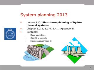
1. System planning 2013 • Lecture L10: Short term planning of hydro-thermal systems • Chapter 5.2.5, 5.3.4, 5.4.1, Appendix B • Contents: • Dual variables • GAMS, example • Home assignment 3

2. Dual variables • LP problem on standard form: • The solution of the problem will result (except of the optimal solution itself) in one dual variable per constraint • The dual variables are measurements of how much the objective function will change if the right-hand side of the constraints are changed

3. 3 x1+x2 7 Dual variables x 2 4 z = 40 3 z = 30 z = 20 2 In optimum: 1 > 0 (active) 2 > 0 (active) 3 = 0 (not active) 1 x2  0 x x1  0 1 1 2 3 4 4x1+12x2 12 x1+x2 2 2 1

4. 1 2 Dual variables • Hydrological constraints: • Hydrological constraints have units HE • Objective function has unit currency (SEK, $, £ ...) • Increase of V more water available  larger income/more stored water  optimal objective value increase The dual variables corresponds the water value [SEK/HE].

5. Dual variables • Contracted load constraints for hour t: • Constraints have unit MWh • Objective function has unit SEK • Increase of Dk increased production cost or less water available at end of planning period  optimal objective function value decreases Dual variables correspond the marginal cost for production, i.e. the power price [SEK/MWh].

6. 1 2 Dual variables - Example • Assume hydropower planning for 6 hours. • The hydro system consists of 2 power stations. • The problem includes contracted load constraints. • Solving the problem resulted in the following dual variables: • 82.4304 hydr. balance for station 1, k = 1,...,6 • 42.6585 hydr. balance for station 2, k = 1,...,6 • -190.0389 load balance, k = 1,2,3,5,6 • -200.0410 load balance, k = 4 • Questions: • What can be said about the structure of the hydro system? • Assume that a customer want to buy another 5 MWh hour 2. How high must the price be for this to be profitable for the producer?

7. Home assignment 2 • Short term hydro-thermal planning • Solved by using the software GAMS (www.gams.com)

8. GAMS • Software specialized for solving optimization problems. • Typical structure of GAMS program: • Define sets • Define parameters • Declare optimization variables • Declare equations • Define equations • Define variable limits

9. 1 2 Example • Two power stations, Degerforsen (1) and Edensforsen (2). • Have sold power to the power exchange. Contracted load for the next 6 hours: 90, 98, 104, 112, 100,80 MWh. • Reservoirs filled to 80% at the beginning • Stored water can be used at best efficiency and power generated in the future can be sold for 185 SEK/MWh. • Neglect the delay time between stations Known:

10. Example

11. Example • Known parameters: • Calculated parameters: • Optimization variables: = discharge, station i, segment j, during hour t, i=1,2, j=1,2, t=1,...,6 = spillage, station i, during hour t, i=1,2, j=1,2, t=1,...,6 = reservoir contents, station i, end of hour t, i=1,2, j=1,2, t=1,...,6

12. Example • Objective: • Constraints:

13. Example • Variable limits:

14. GAMS Sets i power stations /Degerforsen, Edensforsen/ j segments/segment1*segment2/ t time/hour1*hour6/ ; Parameters Mmax(i) maximum contents /Degerforsen 5e6 Edensforsen 4e6/ lambdaf future price /185/ w(i) mean flow /Degerforsen 163 Edensforsen 164/

15. GAMS D(t) contracted load /hour1 90, hour2 98, hour3 104, hour4 112, hour5 100, hour6 80/ Qmax(i,j) maximum discharge station i segment j /Degerforsen.segment1 225, Degerforsen.segment2 75, Edensforsen.segment1 202.5, Degerforsen.segment2 67.5/ mu(i,j) prod equivalent station i segmen j /Degerforsen.segment1 0.209, Degerforsen.segment2 0.199 Edensforsen.segment1 0.236 Degerforsen.segment2 0.224/ V(i) local inflow Mstart(i) start contents of reservoir i ;

16. GAMS Mmax(i) = Mmax(i)/3600; V(i) = w(i)-w(i-1); Mstart(i) = 0.5*Mmax(i); Positive variables Q(i,j,t) discharge station i, segment j, hour t S(i,t) spillage station i, hour t M(i,t) reservoir contents station i, hour t ; Free variable z objective value of stored water ;

17. GAMS equation types

18. GAMS Equation objfnc objective function; objfnc.. z =e= lambdaf*((mu(”Degerforsen”,”segment1”) + mu(”Edensforsen”,”segment1”))*M(”Degerforsen”, ”hour6”) + mu(”Edensforsen”,”segment1”)* M(”Edensforsen”,”hour6”)) ;

19. GAMS Equations hydbal(i,t) Hydrological balance constraints loadbal(t) Load balance constraints ; hydbal(i,t).. M(i,t) =e= M(i,t-1) + Mstart(i)$(ord(t)=1) – sum(j,Q(i,j,t)) – S(i,t) + sum(j,Q(i-1,j,t)) – S(i-1,t) + V(i); loadbal(t).. sum((i,j),mu(i,j)*Q(i,j,t)) =e= D(t);

21. GAMS Q.up(i,j,”hour1”) = Qmax(i,j); M.up(i,”hour1”) = Mmax(i); etc... Alternatively: loop(t,Q.up(i,j,t) = Qmax(i,j); M.up(i,t) = Mmax(i));

22. GAMS model hydroplanning /all/; solve hydroplanning using lp maximizing z; Structuring output: Parameters Qtot(i,t) total discharge per station and hour H(i,t) power production per station and hour ; loop((i,t), Qtot(i,t) = sum(j,Q.L(i,j,t)); H(i,t) = sum(j,mu(i,j)*Q.L(i,j,t))); display M.L, Q.L, Qtot, H, S.L; display hydbal.M, loadbal.M;

23. Discharge plan