Cutting complete weighted graphs
Cutting complete weighted graphs. Math/CSC 870 Spring 2007. Jameson Cahill Ido Heskia. Let be a weighted graph with an Adjacency weight matrix. Our goal: Partition V into two disjoint sets A and B such that the nodes in A (resp. B)

Cutting complete weighted graphs
E N D
Presentation Transcript
Cutting complete weighted graphs Math/CSC 870 Spring 2007 • Jameson Cahill • Ido Heskia
Let be a weighted graph with an Adjacency weight matrix Our goal: Partition V into two disjoint sets A and B such that the nodes in A (resp. B) are strongly connected (=“similar”) to each other, but we would also like to have that the nodes In A are not strongly connected to the Nodes in B. (Then we can continue partition A and B in the same fashion).
To do this we will use the normalized cut Criterion: (We normalize in order to deal with the cuts which favor small isolated sets of points.)
Normalized Cut Criterion: We wish to minimize this quantity across all Partitions
If we let: Then a straightforward calculation shows that (since ) So MinimizingNcut(A,B) simultaneously MaximizesNasso(A,B)!
Bad News: Prop. (Papadimitrou, `97): Normalized Cut for a graph on regular grids is NP hard!! However, good approximate solutions can be found in O(mn) (n=# of nodes, m=max # of matrix-vector computations required) (Use Lanczos Algorithm to find eigen vectors) (linear programming vs. integer programming)
Algorithm: Input: Weighted adjacency matrix (or data file to weigh into an adjacency matrix). Suppose Define a diagonal matrix D by (the degree Of node i) For notational convenience we will write
Let x be an nx1 vector where Now define: So we are looking for the x vector that minimizes this quantity.
Through a straightforward (but hairy) calculation, Shi and Malik show that this Boils down to finding a vector y that minimizes: Where the components of y may take on real Values. This is why our solution is Only approximate (and not NP hard).
The above expression is knows as a Rayleigh quotient and is equivalent to finding a y that minimizes: Which we can rewrite as: Where (Makes sense, since diagonal & pos. entries)
Thus, we just need to find the eigen vector Corresponding to the smallest nonzero Eigen value of the matrix “Thresholding”: For each we have where
We are using this code for the Normalized cut: function [NcutDiscrete,NcutEigenvectors,NcutEigenvalues] = ncutW(W,nbcluster); % [NcutDiscrete,NcutEigenvectors,NcutEigenvalues] = ncutW(W,nbcluster); % % Calls ncut to compute NcutEigenvectors and NcutEigenvalues of W with nbcluster clusters % Then calls discretisation to discretize the NcutEigenvectors into NcutDiscrete % Timothee Cour, Stella Yu, Jianbo Shi, 2004 % compute continuous Ncut eigenvectors [NcutEigenvectors,NcutEigenvalues] = ncut(W,nbcluster); % compute discretize Ncut vectors [NcutDiscrete,NcutEigenvectors] =discretisation(NcutEigenvectors);
Example: Cutting a K5 graph. W: Pair-wise similarity matrix Change all weights into 0 and 1 in order to Draw the graph (for matlab). – but bad output for large number of nodes) – drawgraph(garden).bmp only 400 vertices Transform indicator matrix into adjacency matrix in order to graph. (adjancy_2.m) Load: Desktop\cluster\cluster\matgraph\matgraph\ \example.fig run: load Example.txt; drawgraph(Example); drawgraph_2(Example)
Bad output format for many nodes (here’s example for just 400 nodes and 79,800 edges):
Let’s Cut the Forest… Tropical Rain Forest Pasoh Forest Reserve, Negeri Sembilan, Malaysia. Complete survey of all species of trees for each 5x5 meter square.
The Data File: (cluster\bci5\bci5.dat) 20,000 rows, 303 columns. 1st 2 columns are x,y coords. 301 columns of species. Every 100 rows, x incremented. 200x100 squares each is a 5x5 meters. (1000x500 meter forest)
Model Each square is a node (vector of coords and 301 species). Create an adjacency matrix and the weight w(i,j) Quantifies how “similar” the nodes are.
Similarity indices Pick your favorite weighting function: Weight_1.m Weight_can.m Source: [7]
Trying to weigh a 20,000x20,000 matrix • takes a really long time!!! • So we decided between 2 options • (until finding a REAL machine): • Cut a much smaller piece. • +(learn about presenting output) • 2) Change the “resolution”. • +(cut the whole thing)
Cutting a smaller piece(a garden)… Change the original data file to 400 rows (nodes) instead of 20000. By the way the rows are ordered can’t just take the first 400 rows (otherwise you get a thin strip of 100X4 squares). Take 20 rows and jump by 80 rows until you get 400 rows). (littleforest.dat)
Result: (load garden.txt) or littleforest+weigh+diagonal cut_garden = Ncutw(garden,2) [p1,p2]=firstcut(garden) (coords vector 400x2) [v1,v2]=vector(p1)(1 vector rep. row, 2nd vector rep. column) [v3,v4]=vector(p2) Scatter(v1,v2,’b’), hold on, scatter(v3,v4,’m’)
reweigh_3(cut_garden,garden) – 4 regions [a1,a2,a3,a4,a5,a6,a7,a8] = reweigh_3(Cut,weighted_matrix) So we can make it work for 20x20. Quite easy to generalize it, so number of regions is a parameter. Now we wanted to cut the whole forest and analyze our results.
2) Change of resolution In-stead of looking at 5x5 squares, we can look at a 10x10 meter square (not so bad resolution) and cut the whole forest? So we’ll have a 5,000x5,000 matrix. From original file: add any 2 consecutive Rows and basically jump by 100 to add next row (resolution.m)
Weighting takes only a few hours now, but the RAM fails to deliver! Can’t keep the 5,000x5,000 matrix and do operations on it. (just changing diagonal to 0 takes a long time). (A.txt) Still can’t cut it – get memory errors!!! (can’t even perform the check for symmetry of matrix)
Sensitivity analysis/other stuff to do Somehow cut the whole forest. Compare the cuts we get with the original data. Do the regions indeed consist of similar nodes? Which weight function gave us the “best” cut (compared to the actual data)?
Average out the regions, and see if they are really different than the other Regions. After deciding what was the best cut, we want to start “throwing off data” (change resolution for example) And see how far from the desired cut we get (next survey, how accurate should it be?)
Assuming our results are “good”: Take another look at the data file. Anything special about it that made it Possible to apply image segmentation Techniques on it? What properties of the data file made it “segmentable” using this method?
References: • [1] IEEE Transactions on patterns analysis and machine intelligence vol. 22 no. 8 • Normalized cuts and Image Segmentation. • By Jianbo Shi and Jitendra Malik • [2] Fast Multiscale Image Segmentation. • By Eitan Sharon, Achi Brandt and Ronen Basri. • [3] Nature • Hierarchy and adaptivity in segmenting visual scenes. • By Eitan Sharon, Meirav Galun, Dahlia Sharon, Ronen Basri and Achi Brandt
[4]Tutorial Graph Based Image Segmentation Jianbo Shi, David Martin, Charless Fowlkes, Eitan Sharon http://www.cis.upenn.edu/~jshi/GraphTutorial/Tutorial-ImageSegmentationGraph-cut1-Shi.pdf [5]Normalized Cut image segmentation and data clustering MATLAB code http://www.cis.upenn.edu/~jshi/ [6]Scale dependence of tree abundance and richness in a tropical rain forest, Malaysia. Fangliang He, James V.LaFrankie Bo Song [7] Choosing the Best Similarity Index when Performing Fuzzy Set Ordination on Abundance Data Richard L. Boyce