Nondecreasing Paths in Weighted Graphs
Carnegie Mellon University. SODA 2008. Nondecreasing Paths in Weighted Graphs. Or: How to optimally read a train schedule. Virginia Vassilevska. Tomorrow after 8am. As early as possible!. Traveling?. Routes with Multiple Stops. Los Angeles. Chicago. 10:35pm – 12:35am. 5:05pm – 9:35pm.

Nondecreasing Paths in Weighted Graphs
E N D
Presentation Transcript
Carnegie Mellon University SODA 2008 Nondecreasing Paths in Weighted Graphs Or: How to optimally read a train schedule Virginia Vassilevska
Tomorrow after 8am As early as possible! Traveling?
Routes with Multiple Stops Los Angeles Chicago 10:35pm – 12:35am 5:05pm – 9:35pm 8:35am – 11am 11:40pm – 1:25am Las Vegas BWI 1:30pm – 4pm 7:00pm – 8:45pm 4pm – 8:30pm 1:30pm – 6:00pm
Scheduling • You might need to make several connections. • There are multiple possible stopover points, and multiple possible schedules. • How do you choose which segments to combine?
Los Angeles Chicago Las Vegas BWI Graph-Theoretic Abstraction … … … 10:35pm A vertex for each flight; … 12:35am 10:35pm 9:35pm 1:25am 5:05pm 11:40pm 8:35am 9:30pm 8:30pm 4pm 11am 12pm 8:45pm 1:30pm 4pm 5pm 7pm 1:30pm 6pm 7pm Graph: Nondecreasing path with minimum last edge? (flight, Destination) edges; (Origin, flight) edges; departure time weight; A vertex for each city/airport; arrival time weight;
Versions of the problem Single source – single destination Single source (every destination) Single source (every destination) – SSNP All pairs All pairs – APNP S T
History • G. Minty 1958: graph abstraction and first algorithm for SSNP – polytime • E. F. Moore 1959: a new algorithm for shortest paths, and SSNP – cubic time
m – number of edges n – number of vertices History • Dijkstra 1959 • Fredman and Tarjan 1987 – Fibonacci Heaps implementation of Dijkstra’s; until now asymptotically fastest algorithm for SSNP. O(m+n log n) • Nowadays – experimental research on improving Dijkstra’s algorithm implementation
Our contributions • Linear time algorithm for SSNP in the word-RAM model, O(m log log n) in comparison based model • First truly subcubic algorithm for APNP
Talk Outline • SSNP: • Two known algorithms • A new O(m log log n) algorithm • Linear time algorithm (on a RAM) • APNP: • Brief outline of our approach
d[u] u S SSNP - Dijkstra’s algorithm • Set U = V and T = { }. • At each iteration, pick u from U minimizing d[u]. • T = T U {u}, U = U \ {u}. • For all edges (u, v), • If w(u,v) ≥ d[u], set d[v] = min (d[v], w(u,v)) Iterate: Iterate: T w(u,v) min d[u] v U
Running time of Dijkstra • Using Fibonacci Heaps, Dijkstra can be implemented in O(m+n log n) time. • Optimal for Dijkstra’s algorithm – nodes visited in sorted order of their distance. • The bottleneck are the n extract-mins.
N(F) F More on Dijkstra’s • Suppose we only maintain F vertices in the Fibonacci heaps. The rest we maintain in some other way. • Then the runtime due to the Fibonacci heaps would be O(F log F + N(F)) where N(F) is the number of edges pointing to the F vertices. • For F = m/log n, this is O(m)!
v u ALG2: Depth First Search - Like DFS(v, d[v]): For all (v, u) with w(v, u) ≥ d[v]: Remove (v, u) from graph. d[u] = min (d[u], w(v,u)) DFS(u, d[u]) d[S] = - ∞, start with DFS(S, d[S]). d[v]=2 1 3 3 d[u]=4 d[u]=3
Naive Runtime of DFS • The number of times we call DFS(v, d[v]) for any particular v is at most indegree(v). • Every such time we might have to check all outedges (w(v,u)≥?d[v]). • Worst case running time: O(mn).
More on DFS • Suppose for a node v and weight d[v] we can access each edge (v, u) with w(v, u)≥ d[v] in O(t) time. • As each edge is accessed at most once, the runtime is O(m t). • For each node, store its neighbors in a binary search tree w.r.t. outgoing weights. O(m log n) runtime
High Degree Low Degree Combine Dijkstra with DFS • Recall: • If F nodes used in Fibonacci heaps, then the Dijkstra runtime due to the heaps is O(F log F + N(F)) • If DFS with binary search trees is run on a set of nodes T, the runtime is O(Σv T { degin(v) log (degout(v)) }) O(m log log n) for T = {v | degout(v)<log n} ◄ O(m+n) for F = m/log n {v | degout(v) ≥ log n}
Idea Summary • Run DFS on vertices of low degree < log n: O(m log log n) time. • Put the O(m/log n) high degree nodes in Fibonacci heaps and run Dijkstra on them. Time due to Fibonacci heaps: O(m). • We get O(m log log n). Better than O(m+n log n) for m = o(n log n/log log n).
RAM But we wanted linear time… Fredman and Willard atomic heaps: • After O(n) preprocessing, a collection of O(n) sets of O(log n) size can be maintained so that the following are in constant time: • Insert • Delete • Given w, return an element of weight ≥ w. outedges of low degree vertices
Linear runtime • Replace binary trees by atomic heaps. • Time due to Dijkstra with Fibonacci Heaps on O(m/log n) elements is still O(m). • Time due to DFS with atomic heaps: • inserting outedges into atomic heaps takes constant time per edge; • given d[v], accessing an edge with w(v,u) ≥ d[v] takes constant time. • O(m+n) time overall! But how do we combine Dijkstra and DFS?
Linear Time Algorithm • Stage 1: Initialize • Find all vertices v of degree ≥log n and insert into Fibonacci Heaps with d[v] = ∞; • For all vertices u of degree < log n, add outedges into atomic heap sorted by weights. • This stage takes O(m+n) time. Insert S with d[S] = - ∞
Linear Time Algorithm Cont. • Stage 2: Repeat: • Extract vertex v from Fibonacci heaps with minimum d[v] • For all neighbors u of v, if w(u,v) ≥ d[v]: • Update d[u] if w(v,u) < d[u] • Run DFS(u, d[u]) on the graph spanned by low degree vertices until no more can be reached • If Fib.heaps nonempty, go to 1. Fibonacci Heaps 2 2 3 3 4 5 1 4 4
4 7 0 9 i j 4 5 All Pairs Nondecreasing Paths (APNP) • (min, ≤ )-matrix product C = A • B: C[i, j] = mink { B[k, j] | A[i, k] ≤ B[k, j] } • (( W • W) • W) … • W) - min nondecreasing k times Say W is the adjacency matrix: W[i, i] = - and W[i ,j] = w(i, j) for i ≠ j. A B paths of length ≤ k
All Pairs Nondecreasing Paths cont. • We give an algorithm for (min, ≤ )-product of n x n matrices running in O(n2.8) time. • Hence, APNP for paths of length at most k can be done in O(k n2.8) time. • We show how to find APNP for paths of length at least k in Õ(n3 / k) time. • → O(n2.9) Algorithm for APNP.
Summary • We gave the first linear time algorithm for the single source nondecreasing paths problem, and the first subcubic algorithm for APNP. • Now you can read a train schedule optimally!
w’1 … w1 0 w’1 d d’ … … … w1 … d’ d … 0 0 w’d’ wd 0 w’d’ wd Directions for future work • Single source shortest paths? • Our degree approach fails – finding a linear time algorithm is hardest on low degree graphs • Shortest Nondecreasing Paths? o(m log n)?
The End. THANK YOU!
Example U - Fibonacci Heap: S: -infinity P: infinity Q: infinity 2 S 3 c 1 5 4 3 b a Other Distances: a: infinity b: infinity c: infinity d: infinity 3 2 Q 3 5 P 2 2 d 3
Example U - Fibonacci Heap: P: infinity Q: infinity 2 S 3 c 1 5 4 3 b a Other Distances: a: 5 b: 1 c: 3 d: infinity S: -infinity 3 2 Q 3 5 P 2 2 d 3 S – extract min from U
Example U - Fibonacci Heap: P: 2 Q: infinity 2 S 3 c 1 5 4 3 b a Other Distances: a: 5 b: 1 c: 3 d: infinity S: -infinity 3 2 Q 3 5 P 2 2 d 3 DFS(b, 1)
Example U - Fibonacci Heap: P: 2 Q: infinity 2 S 3 c 1 5 4 3 3 b a Other Distances: a: 5 b: 1 c: 3 d: infinity S: -infinity 3 2 Q 3 5 P 2 2 d 3 DFS(c, 3) DFS(a, 5)
Example U - Fibonacci Heap: Q: 3 2 S 3 c 1 5 4 Other Distances: a: 3 b: 1 c: 3 d: 2 S: -infinity P: 2 3 b a 3 2 Q 3 5 P 2 2 d 3 P – extract min from U
Example U - Fibonacci Heap: Q: 3 2 S 3 c 1 5 Other Distances: a: 2 b: 1 c: 3 d: 2 S: -infinity P: 2 4 3 b a 3 2 Q 3 5 P 2 2 d 3 DFS(d, 2)
Example U - Fibonacci Heap: Q: 3 2 S 3 c 1 5 Other Distances: a: 2 b: 1 c: 2 d: 2 S: -infinity P: 2 4 3 b a 3 2 Q 3 5 P 2 2 d 3 DFS(a, 2)
Example U - Fibonacci Heap: Q: 3 2 S 3 c 1 5 Other Distances: a: 2 b: 1 c: 2 d: 2 S: -infinity P: 2 4 3 b a 3 2 Q 3 5 P 2 2 d 3 DFS(a, 3) DFS(c, 2)
Example U - Fibonacci Heap: 2 S 3 c 1 5 Other Distances: a: 2 b: 1 c: 2 d: 2 S: -infinity P: 2 Q: 3 4 3 b a 3 2 Q 3 5 P 2 2 d 3 Q – extract min from U
New York London Atlanta Paris 11:35pm – 1pm 7:45pm – 8:30pm Newark Frankfurt 11:40am – 4:15pm 7pm – 1:20pm 5:30pm – 10:40am
Graph-Theoretic Abstraction • City vertices and Train vertices • Edges between origin and train and train and destination • Weight on origin -> train edge is departure time • Weight on train -> destination edge is arrival time
Fibonacci Heaps • Inserting n vertices initially takes O(n) time. • Updating the distance d[v] of a vertex v takes constant time. • Returning the vertex u minimizing d[u] takes logarithmic time.