Cutting Complete Weighted Graphs for Image Segmentation in Computer Vision
This paper discusses the application of complete weighted graphs in image segmentation, aiming to partition images into regions based on pixel similarities. Each pixel is represented as a node in a graph, with edges weighted according to their similarity. The main objective is to minimize the total weight of edges cut between clusters of nodes, ensuring high similarity within clusters and low similarity across different clusters. The method employs normalized cuts and introduces a weighted aggregation algorithm to optimize the segmentation process for various applications, including forest species classification.

Cutting Complete Weighted Graphs for Image Segmentation in Computer Vision
E N D
Presentation Transcript
Cutting complete weighted graphs Math/CSC 870 Spring 2007 • Jameson Cahill • Ido Heskia
Cutting Complete Weighted Graphs In image segmentation in computer vision the goal is to divide the image into regions which are similar in the properties of the pixels. Image is a weighted graph Nodes are the pixels. Each pixel has a vector associated to it Containing the data about the properties of the pixel (texture, color, intensity, etc).
Image segmentation: basic model We start with a complete graph (an edge between every 2 nodes) The weight of the edge w(i,j) corresponds to the similarity between nodes i,j. The more the nodes are “similar” the higher the weight that is associated to the edge joining them.
Goal: Partition V into disjoint sets of nodes V1,…, Vm In such a way that the similarity between the nodes in each set Vi is high and across different sets Vi,Vj is low. We partition the nodes, so that However, we are about to lose edges, since we are cutting our graph.
Cutting graphs T1 T2 A 7 X 5 1 2 6 4 3 C B 4 Z Y We could cut this graph by removing the edges (A,X) and (C,Y) whose weights are 7 and 4 respectively. The In this case it is =11 +
So we can partition by removing edges that connect 2 components. To make sure the regions are indeed different we’re looking for edges whose weight is low, so we wish to minimize the total weight of the edges that have been removed. Minimize the cut Unfortunately, it is not that simple. Example:
Imagine that there are weighted edges between each pair of nodes. Assume that the similarity between nodes in this case is simply their Euclidean distance from each other so the weights of the edges between close nodes is high. We want to bipartition this graph. Bad cut Best cut Since we are simply minimizing the cut, we will actually pick the bad cut in this case since any edge we add on to the cut increases it. We must Normalize this cut!
Normalized cuts Calculate the cut as a fraction of the total edge connections from the set to the rest of the graph to exclude cuts of small isolated Components, called the Ncut. disassociation measure. Now the previous cut which favors small isolated sets won’t have low Ncut value since it will be a large percentage of the total connections From that set to all other nodes (in the previous example it will be 100%).
Normalized association The measure for similarity between sets of nodes (Nassoc): Where This gives us the measure of how closely related (on average) nodes within the set A are, relatively to their similarity to the rest of the nodes in the graph.
We have this relationship between these measures: Thus, when we try to minimize the Ncut we also maximize the Nassoc and we indeed make sure that the two requirements we imposed on our partition of the nodes will be satisfied. Now we could apply this to our complete graph, and continue recursively on each component until we get Our desired m components.
What’s the plan We plan to study an algorithm inspired by algabraic multi-grid which involves the normalized cuts. Basics of the segmentation by weighted aggregation (SWA) algorithm: We are treating our graph as a grid graph, starting from the most Refined grid, and we coarsen it at each step. First choose ½ your nodes as representatives (called seeds). Choose those so that each node in your graph is “strongly” connected to at-least one seed adjacent to it.
Aggregation Now we will aggregate all the nodes which are strongly coupled to a seed, to that respective seed, so that we eliminate a big amount of the nodes. Now each node Corresponds to an aggregate of pixels, not just a single one. • Recalculate the aggregate properties. • Recalculate the edges weight accordingly. • Now apply the same to the seeds.
This process only keeps tracks of what are the different regions. In order to find the actual boundaries, we will have to retrace our steps. So what do we want to do?
First we want to understand the SWA algorithm and write a Matlab Code which performs it. We will test our code trying to segment images. If we can make that happen then we would really like to Segment a Forest Each node corresponds to a square of land, and the vector Associated with it records which species of plants are in this square. Similarly to image segmentation, we want to partition the forest into regions which our similar in the species of plants which they consist of.
Refrences: • IEEE Transactions on patterns analysis and machine intelligence vol. 22 no. 8 • Normalized cuts and Image Segmentation. • By Jianbo Shi and Jitendra Malik • Fast Multiscale Image Segmentation. • By Eitan Sharon, Achi Brandt and Ronen Basri. • Nature • Hierarchy and adaptivity in segmenting visual scenes. • By Eitan Sharon, Meirav Galun, Dahlia Sharon, Ronen Basri and Achi Brandt