Download
1 / 16
160 likes | 299 Vues
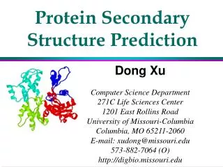
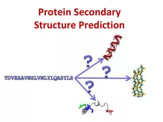
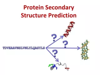
This lecture focuses on the evolution of protein secondary structure prediction methods, highlighting early statistical approaches like Chou-Fasman rules and advancements through neural network models. Notable developments include Qian-Sejnowski's pioneering work on multi-layer perceptrons (MLPs) using contiguous amino acid residues for prediction, which demonstrated improved accuracy over traditional methods. We discuss the integration of evolutionary information and multiple sequence alignments in predictive frameworks, enhancing signal-to-noise ratios. Additionally, strategies to minimize overfitting and optimize predictive performance are covered.

E N D
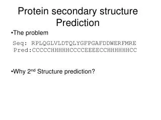
Secondary Structure Prediction • Progressive improvement • Chou-Fasman rules • Qian-Sejnowski • Burkhard-Rost PHD • Riis-Krogh • Chou-Fasman rules • Based on statistical analysis of residue frequencies in different kinds of secondary structure • Useful, but of limited accuracy Lecture 11, CS567
Qian-Sejnowski • Pioneering NN approach • Input: 13 contiguous amino acid residues • Output: Prediction of secondary structure of central residue • Architecture: • Fully connected MLP • Orthogonal encoding of input, • Single hidden layer with 40 units • 3 neuron output layer • Training: • Initial weight between -0.3 and 0.3 • Backpropagation with the LMS (Steepest Descent) algorithm • Output: Helix xor Sheet xor Coil (Winner take all) Lecture 11, CS567
Qian-Sejnowski • Performance • Dramatic improvement over Chou-Fasman • Assessment • Q = 62.7% (Proportion of correct predictions) • Correlation coefficient (Eq 6.1) • Better parameter because • It considers all of TP, FP, TN and FN • Chi-squared test can be used to assess significance • C = 0.35; C = 0.29, Cc = 0.38; • Refinement • Outputs as inputs into second network (13X3 inputs, otherwise identical) • Q = 64.3%; C = 0.41; C = 0.31, Cc = 0.41 Lecture 11, CS567
PHD (Rost-Sander) • Drawback of QS method • Large number of parameters (104 versus 2 X 10⁴ examples) leads to overfitting • Theoretical limit on accuracy using only sequence per se as input~ 68% • Key aspect of PHD: Use evolutionary information • Go beyond single sequence by using information from similar sequences (Enhance signal-noise ratio; “Look for more swallows before declaring summer”) through multiple sequence alignments • Prediction in context of conservation (similar residues) within families of proteins • Prediction in context of whole protein Lecture 11, CS567
PHD (Rost-Sander) • Find proteins similar to the input protein • Construct a multiple sequence alignment • Use frequentist approach to assess position-wise conservation • Include extra information (similarity) in the network input • Position-wise conservation weight (Real) • Insertion (Boolean); Deletion (Boolean) • Overfitting minimized by • Early stopping and • Jury of heterogeneous networks for prediction • Performance • Q = 69.7%; C = 0.58; C = 0.5, Cc = 0.5 Lecture 11, CS567
PHD inputFig 6.2 Lecture 11, CS567
PHD architectureFig 6.2 Lecture 11, CS567
Riis-Krogh NN • Drawback of PHD • Large input layer • Network globally optimized for all 3 classes; scope for optimizing wrt each predicted class • Key aspects of RK • Use local encoding with weight sharing to minimize number of parameters • Different network for prediction of each class Lecture 11, CS567
RK architecture (Fig 6.3) Lecture 11, CS567
RK architecture (Fig 6.4) Lecture 11, CS567
Riis-Krogh NN • Find proteins similar to the input protein • Construct a multiple sequence alignment • Use frequentist approach to assess position-wise conservation • BUT first predict structure of each sequence separately, followed by integration based on conservation weights Lecture 11, CS567
Riis-Krogh NN • Architecture • Local encoding • Each amino acid represented by analog value (‘real correlation’, not algebraic) • Weight sharing to minimize parameters • Extra hidden layer as part of input • For helix prediction network, use sparse connectivity based on known periodicity • Use ensembles of networks differing in architecture for prediction (hidden units) • Second integrative network used for prediction • Performance • Q = 71.3%; C = 0.59; C = 0.5, Cc = 0.5 • Corresponds to theoretical upper bound for a contiguous window based method Lecture 11, CS567
NN tips & tricks • Avoid overfitting (avoid local minima) • Use the fewest parameters possible • Transform/filter input • Use weight sharing • Consider partial connectivity • Use large number of training examples • Early stopping • Online learning as opposed to batch/offline learning (“One of the few situations where noise is beneficial”) • Start with different values for parameters • Use random descent (“ascent”) when needed Lecture 11, CS567
NN tips & tricks • Improving predictive performance • Experiment with different network configurations • Combine networks (ensembles) • Use priors in processing input (Context information, non-contiguous information) • Use appropriate measures of performance (e.g., correlation coefficient for binary output) • Use balanced training • Improving computational performance • Optimization methods based on second derivatives Lecture 11, CS567
Measures of accuracy • Vector of TP, FP, TN, FN is best, but not very intuitive measure of distance between data (target) and model (prediction), and restricted to binary output • Alternative: Single measures (transformation of above vector) • Proportions based on TP, FP, TN, FN • Sensitivity (Minimize false negatives) • Specificity (Minimize false positives) • Accuracy (Minimize wrong predictions) Lecture 11, CS567
Measures of error/accuracy • Lp distances (Minkowski distances) • (i |di - mi|p )1/p • L1 distance = Hamming/Manhattan distance = i |di - mi| • L2 distance = Euclidean/Quadratic distance = (i |di - mi|2 )1/2 • Pearson correlation coefficient • I (di – E[d])(mi - E[m])/d m • (TP.TN – FP.FN)/(TP+FN)(TP+FP)(TN+FP)(TN+FN) • Relative entropy (déjà vu) • Mutual information (déjà vu aussi) Lecture 11, CS567