Real Time PCR Quantitative PCR
Real Time PCR Quantitative PCR. PCR: P olymerase C hain R eaction. … a method widely used in molecular biology to make many copies of a specific DNA segment. In general is an exponential amplification. # copies = 2 n.


Real Time PCR Quantitative PCR
E N D
Presentation Transcript
Real Time PCR Quantitative PCR
PCR: Polymerase Chain Reaction … a method widely used in molecular biology to make many copies of a specific DNA segment In general is an exponential amplification # copies = 2n After each cycle , the amount of DNA is twice what it was before, after N cycles we shall have 2n times as much. But, of course, the reaction cannot go on forever, and it eventually tails off and reaches a plateau phase. 2(21) 4(22) 8(23)
Phases of a PCR reaction three phases The exponential phase is the period in which exact doubling of a nucleic acid product occurs every cycle. The linear phase occurs as the reaction is slowing due to the consumption of the reagents and the degradation of the products. The final stage is the plateau phase, which occurs when the reaction has stopped, and no additional amplicon is being generated. This is the point at which the PCR reaction product is analyzed via gel electrophoresis for conventional PCR reactions. BUT is there a quantitative relationshipbetween amount of starting target sequence and amount of PCR product at any given cycle? NO
DAY2 28 cycles NO it is a common experience for replicate reactions to yield different amounts of PCR product A B C D 28 cycles DAY1 rtPCR_ expression level Semi-quantitative PCR Quantitative PCR Real Time-PCR
Quantitative or real time-PCR (qPCR/RT-PCR) qPCR combine ‘traditional’ end-point detection PCR fluorescent detection technologies to record the accumulation of amplicons in ‘real time’ during each cycle of the PCR amplification. Detection of amplicons occurs during the early exponential phase of the PCR this enables the quantification of gene numbers when these are proportional to the starting template concentration.
History of qPCR 1993 Higuchi et al. uses a video camera to monitor multiple polymerase chain reactions (PCRs) simultaneously over the course of thermocycling. ‘traditional’ end-point detection PCR The video camera detects the accumulation of double-stranded DNA (dsDNA) in each PCR using the increase in the fluorescence of ethidium bromide (EtBr) that results from its binding duplex DNA. fluorescent detection technologies
qPCR overwiew The real-time PCR system is based on the detection and quantitation of a fluorescent reporter. This signal increases in direct proportion to the amount of PCR product in a reaction. By recording the amount of fluorescence emission at each cycle, it is possible to monitor the PCR reaction during exponential phase where the first significant increase in the amount of PCR product correlates to the initial amount of target template (during the exponential phase, the amount of PCR product approximately doubles in each cycle). As the reaction proceeds, however, reaction components are consumed, and ultimately one or more of the components becomes limiting. At this point, the reaction slows and enters the plateau phase Initially, fluorescence remains at background levels, and increases in fluorescence are not detectable (cycles 1-18) even though product accumulates exponentially Eventually, enough amplified product accumulates to yield a detectable fluorescent signal. The cycle number at which this occurs is called the threshold cycle, or CT
qPCR overwiew In conclusion, the parameter CT (threshold cycle) is defined as the cycle number at which the fluorescence emission exceeds the fixed threshold; the higher the starting copy number of the nucleic acid target, the sooner a significant increase in fluorescence is observed. Thus, the reaction will have a high, or late, CT and vice versa Chemistry developments for REAL-TIME PCR Double-Stranded DNA Binding Dyes (Intercalator-based) Fluorogenic Probes hydrolysis probes hybridizing probes
Chemistry developments for REAL-TIME PCR TaqMan probes,molecular beacons and scorpions. Fluorogenic Probes hydrolysis probes hybridizing probes TaqMan probes use the exonuclease activity of Taq polymerase to measure the amount of DNA target sequences in samples oligonucleotides longer than the primers (20-30 bases long with a Tm value of 10 oC higher) that contain a fluorescent dye usually on the 5' base. a quenching dye (usually TAMRA or a non-fluorescent quencher) typically on the 3' base. designed to anneal to an internal region of a PCR product. TaqMan probes When irradiated, the excited fluorescent dye transfers energy to the nearby quenching dye molecule rather than fluorescing (this is called FRET = Förster or fluorescence resonance energy transfer). the close proximity of the reporter and quencher prevents emission of any fluorescence while the probe is intact
Chemistry developments for REAL-TIME PCR Fluorogenic Probes hydrolysis probes hybridizing probes TaqMan probes When the polymerase replicates a template on which a TaqMan probe is bound, its 5' exonuclease activity cleaves the 5’ end of probe which contains the reporter dye. This ends the activity of quencher (no FRET) and the reporter dye starts to emit fluorescence which increases in each cycle proportional to the rate of probe cleavage. Accumulation of PCR products is detected by monitoring the increase in fluorescence of the reporter dye (note that primers are not labeled). Because the cleavage occurs only if the probe hybridizes to the target, the origin of the detected fluorescence is specific.
Chemistry developments for REAL-TIME PCR Fluorogenic Probes hybridizing probes Molecular Beacons also contain fluorescent (FAM, TET, ROX) and quenching dyes (typically DABCYL or BHQ) at either end they are designed to adopt a hairpin structure while free in solution to bring the fluorescent dye and the quencher in close proximity for FRET to occur.
Chemistry developments for REAL-TIME PCR Fluorogenic Probes hybridizing probes Molecular Beacons When the beacon hybridizes to the target during the annealing step, the reporter dye is separated from the quencher and the reporter fluoresces (FRET does not occur) During the extension step, when the temperature is raised (approximately 72°C) to promote DNA synthesis, the temperature is too high for the molecular beacons to remain on their target sequences, so the molecular beacons fall off of their targets and do not interfere with polymerization Molecular beacons remain intact during PCR and must rebind to target every cycle for fluorescence emission. This will correlate to the amount of PCR product available
Chemistry developments for REAL-TIME PCR Fluorogenic Probes hybridizing probes Scorpion probes bi-functional molecules that carry both probe and priming functions on the same oligonucleotide construct The probe element is attached as a tail to the primer element through a PCR blocker thatensures the probe element does not get incorporated into the double-stranded product The primer element binds to the DNA target; the probe element is in the closed, non-fluorescent configuration. Upon subsequent rounds of heating and cooling, the extension product becomes single stranded and the probe can bind to its complement in a rapid intramolecular rearrangementand. the fluorophore becomes unquenched leading to an increase in specific fluorescence.
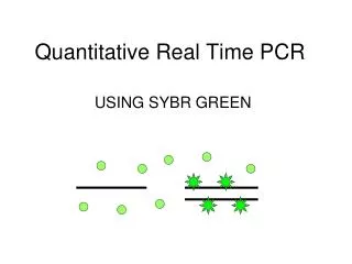
Chemistry developments for REAL-TIME PCR Double-Stranded DNA Binding Dyes (Intercalator-based) The cheaper alternative to the probes is the double-stranded DNA binding dye chemistry by the use of a non-sequence specific fluorescent intercalating agent (SYBR-green I or ethidium bromide). Sybr Green I SYBR green does not bind to ssDNA. is a fluorogenic minor groove binding dye exhibits little fluorescence when in solution but emits a strong fluorescent signal upon binding to double-stranded DNA.
Chemistry developments for REAL-TIME PCR DISADVANTAGE ADVANTAGE • different probes must be synthesized to detect different sequences • specific hybridization between probe and target is required to generate fluorescent signal Fluorogenic Probes • can be labeled with different, distinguishable reporter dyes. • expensive • the dye allows detection of any double-stranded DNA generated during PCR • the dye allows detection of any double-stranded DNA generated during PCR dsDNA Binding Dyes • the same dye can be used to detect any amplified product including non-specific amplification and primer-dimer complex non-specific amplifications require follow-up assays (melting point or dissociation curve analysis) for amplicon identification
qPCR overwiew dsDNA Binding Dyes Fluorogenic Probes
qPCR overwiew Remember…… dsDNA Binding Dyes In real-time PCR using SYBR green binding to amplified cDNA or DNA , we are simply measuring the fluorescenceincrease as the dye binds to the increasing amount of DNA in the reaction tube. ? Are we sure that this increase in fluorescence is coming from the DNA that we wish to amplify BUT or is the signal from a different DNA than the one we're trying to amplify? • not only monitor DNA synthesis during the PCR • determines the melting point of the product at the end of the amplification reactions The melting temperature of a DNA double helix depends on its base composition. All PCR products for a particular primer pair should have the same melting temperature - unless there is contamination, mispriming, primer-dimer artifacts, or some other problem.
qPCR: Optimization of Real Time PCR dsDNA Binding Dyes Fluorogenic Probes Standard curve (for primer test) Since real-time quantification is based on the relationship between initial template amount and the CT value obtained during amplification, an optimal Real Time PCR assay is absolutely essential for accurate and reproducible quantification of your sample. The hallmarks of an optimized Real Time PCR assay are: • Linear standard curve (R2 > 0.980 – r > 0.990) • High amplification efficiency E (90–105%) • Consistency across replicate reactions
qPCR: Optimization of Real Time PCR 1.Standard curve (for primer test) run serial dilutions of a template and use the results to generate a standard curve To determine if your primers work well template used for this purpose can be a target with known concentration (e.g., nanograms of genomic DNA or copies of plasmid DNA) or a sample of unknown quantity (e.g., cDNA or Input DNA from ChIP assay). The standard curve is constructed by plotting the log of the starting quantity of template (or the dilution factor, for unknown quantities) against the CT value obtained during amplification of each dilution.
qPCR: Optimization of Real Time PCR 1.Standard curve (for primer test) - Ideally, the dilution series will produce amplification curves that are evenly spaced. - If perfect doubling occurs with each amplification cycle, the spacing of the fluorescence curves will be determined by the equation: n is the number of cycles between curves at the fluorescence threshold (in other words, the difference between the CT values of the curves) 2n =dilution factor with a 10-fold serial dilution of DNA, 2n = 10. Therefore (log210=n) n = 3.32 CT values should be separated by 3.32 cycles
qPCR: Optimization of Real Time PCR 1.Standard curve (for primer test) Evenly spaced amplification curves will produce a linear standard curve The r valueof a standard curve represents how well the experimental data fit the regression line, that is, how linear the data are. r > 0.990 A significant difference in observed CT values between replicates will lower the r value.
qPCR: Optimization of Real Time PCR 2.Amplification efficiency (for primer test) Amplification efficiency, E, is calculated from the slope of the standard curve using the following formula: E = 10–1/slope Ideally, the amount of PCR product will perfectly double during each cycle of exponential amplification; that is, there will be a 2-fold increase in the number of copies with each: in this case E=2 2 = 10–1/slope Slope:-3.32 Note that the absolute value of the slope is the same as the ideal spacing of the fluorescent traces described above.
qPCR: Optimization of Real Time PCR 2.Amplification efficiency (for primer test) Amplification efficiency, E, is also frequently presented as a percentage, that is, the percent of template that was amplified in each cycle. To convert E into a percentage: % Efficiency= (E – 1) x 100% For an ideal reaction, % Efficiency = (2 – 1) x 100% = 100%. For the example shown in figure above: E = 10–(1/–3.436) = 1.954 % Efficiency = (1.954 – 1) x 100% = 95.4% At the end of each cycle, the amplicon copy number increased 1.954-fold,or 95.4% of the template was amplified
qPCR: Optimization of Real Time PCR 2.Amplification efficiency (for primer test) Amplification efficiency, E • close to 100% (95-105%) best indicator of a robust, reproducible assay • < to 95% may be caused by poor primer design or by suboptimal reaction conditions may indicate pipetting error in your serial dilutions or co-amplification of non specific products, such as primer-dimers • < to 105%
qPCR: Optimization of Real Time PCR dsDNA Binding Dyes Fluorogenic Probes Primers and amplicon design guidelines Both primers and target sequence affect qPCR efficiency For primer design, follow these parameters:• Design primers with a GC content of 50–60%• Maintain a melting temperature (Tm) between 50ºC and 67ºC. • Avoid secondary structure; adjust primer locations outside of the target sequence secondary structure if required• Avoid repeats of Gs or Cs longer than three bases• Place Gs and Cs on ends of primers• Check sequence of forward and reverse primers to ensure no 3' complementarity (avoid primer-dimer formation) • For amplicon design, follow these guidelines:• Design amplicon to be 75–200 bp. Shorter amplicons are typically amplified with higher efficiency. • An amplicon should be at least 75 bp to easily distinguish it from any primer-dimers that might form
qPCR: Optimization of Real Time PCR dsDNA Binding Dyes The advantages of using dsDNA-binding dyes simple assay design (only two primers are needed; probe design is not necessary) ability to test multiple genes quickly without designing multiple probes (e.g., for validation of gene expression data from many genes in a microarray experiment) lower initial cost (probes cost more) Melting curve possibility to perform a melt-curve analysis to check the specificity of the amplification reaction
qPCR: Optimization of Real Time PCR dsDNA Binding Dyes Melting curve Melt-curve analysis can be used to identifydifferent reaction products, including nonspecific products After completion of the amplification reaction, a melt curve is generated by increasing the temperature in small increments and monitoring the fluorescent signal at each step.
qPCR: Optimization of Real Time PCR dsDNA Binding Dyes Melting curve As the dsDNA in the reaction denatures, the fluorescence decreases. The negative first derivative of the change in fluorescence is plotted as a function of temperature A characteristic peak at the amplicon’s melting temperature(Tm, the temperature at which 50% of the base pairs of a DNA duplex are separated) distinguishes it from other products primer-dimers: melt at different temperatures. The melt peak with a Tm of 89°C represents the specific product, while the peak with a Tm of 78°C represents the non specific product
qPCR assay: components Probes Sybr Green I • qPCR master mix with SYBR Green I• Template• Primers Pre-formulated 2X real-time PCR master mixes containing buffer, DNA polymerase, dNTPs, and SYBR Green I dye and a reference dye (fluorescein/ROX). • qPCR master mix • Template• Primers • Probe Pre-formulated 2X real-time PCR master mixes containing buffer, DNA polymerase, dNTPs and a reference dye (fluorescein/ROX). IMPORTANT!! each sample in triplicate. Remember to consider a triplicate for H2O (neg. control). It is possible to perform a Real Time PCR assay with a final volume of 50ul or 15ul.
#3 #1 #2 Ab -flag #3 #1 #2 #3 Ab -flag #1 #2 Ab -flag qPCR assay Sybr Green I Component Volume per reaction Final concentration qPCR Mastermix 12,5 μl 1X Primer 1 300 nM 100 nM–500 nM Primer 2 300 nM 100 nM–500 nM Sterile water x μl DNA template 2 μl Total Volume up to25 μl INPUT INPUT 1:10 INPUT 1:100 INPUT 1:1000 each sample in triplicate INPUT INPUT 1:10 INPUT 1:100 INPUT 1:1000 INPUT INPUT 1:10 INPUT 1:100 INPUT 1:1000 for standard curve NO TEMPLATE
#3 #1 #2 Ab -flag #3 #1 #2 #3 Ab -flag #1 #2 Ab -flag qPCR assay Sybr Green I INPUT INPUT 1:10 INPUT 1:100 INPUT 1:1000 INPUT INPUT 1:10 INPUT 1:100 INPUT 1:1000 #1 #2 #3 Ab -flag NO TEMPLATE INPUT INPUT 1:10 INPUT 1:100 INPUT 1:1000 INPUT INPUT 1:10 INPUT 1:100 INPUT 1:1000 for standard curve NO TEMPLATE
qPCR data analysis Interpretation of results: absolute and relative quantification Absolute quantificationis achieved by comparing the CT values of the test samples to a standard curve. The result of the analysis is quantity of nucleic acid (copy number, μg) per given amount of sample (per cell, per μg of total RNA/DNA). Inrelative quantificationthe analysis result is a ratio: the relative amount (fold difference) of a target nucleic acid for equivalent amounts of test and control sample (A vs. B) For both absolute and relative quantification methods, quantities obtained from a Real Time PCR experiment must be normalized in such a way that the data become biologically meaningful. This is done through the use of normalizers.
qPCR data analysis Interpretation of results: absolute quantification In absolute quantification, the quantity of the unknown sample is interpolated from a range of standards of known quantity. To construct a standard curve, a template with known concentration is required. Dilution of this template is then performed and these dilutions serve as the standards The standard curve can then be used to determine the target quantity in the unknown sample by interpolation when standards and the samples were then assayed in the same run. The equation for the linear regression line is y = mx + b or CT = m(log quantity) + b Quantity = 10(CT-b)/m
qPCR data analysis Interpretation of results: relative quantification Relative quantification measures the relative change in mRNA expression levels. determines the changes in steady-state mRNA levels of a gene across multiple samples expresses it relative to the levels of another RNA. Relative quantification does not require a calibration curve or standards with known concentrations. The units used to express relative quantities are irrelevant, and the relative quantities can be compared across multiple real-time RT-PCR experiments (Orlando et al., 1998; Vandesompele et al., 2002; Hellemans et al., 2006). Often constant expressed reference genes are chosen as reference genes, which can be co-amplified in the same tube in a multiplexassay (as endogenous controls) or can be amplified in a separate tube (asexogenous controls) (Wittwer et al., 2001; Livak, 1997, 2001; Morse et al.,2005).
qPCR data analysis Interpretation of results: relative quantification To determine the level of expression, the differences (∆) between the threshold cycle (Ct) are measured. Thus the mentioned methods can be summarized as the ∆Ct methods But the complexity of the relative quantification procedure can be increased. In a further step a second relative parameter can be added, e.g. comparing the gene of interest (GOI) expression level relative to: a non treated control a time point zero These more complex relative quantification methods can be summarizedas ∆∆Ct methods (Livak and Schmittgen, 2001) 3 general procedures of calculation of the relative quantificationratio are established
Relative quantification: the “delta Ct “ or “delta delta” Ct method These methods assume that both target and reference genes are amplified with efficiencies near 100% and within 5% of each other Once you have verified that the target and reference genes have similar and nearly 100% amplification efficiencies (by performing a standard curve) 1.the “delta Ct “ How can you determine the relative difference in expression level of your target gene in different samples? the relative expression ratio (R) normalize the CT of the target gene(tg) to that of the reference gene(rg), ∆CT = CT(tg) – CT(rg) calculate the expression ratio 2–∆CT = relative expression ratio (R)
Relative quantification: the 2–∆CT method An example To better understand, cDNA representing total RNA isolated from not treated(nt) cells were assayed for NF-YB (target gene (tg)) and GAPDH (reference gene(rg)). • - normalize the CT of the target gene(tg) NF-YB to that of the reference gene(rg) GAPDH, for both the not treated and treated sample: • ∆CT(t) = 12,00 – 15,90 = -3,90 • calculate the expression ratio: • 2–∆CT = 2-(-3,90) = 14,9 =R the relative expression ratio (R) of NF-YB is 14.9-fold higher than reference gene.
2.the “delta delta Ct “ How can you determine the relative difference in expression level of your target gene in different samples? Comparison between nt and t samples normalize the CT of the target gene(tg) to that of the reference gene(rg), for both the not treated(nt) and treated(t) sample ∆CT(t) = CT(tg, t) – CT(rg, t) ∆CT(nt) = CT(tg, nt) – CT(rg, nt) normalize the ∆CT of (t) sample to the ∆CT of the (nt) sample ∆∆CT = ∆CT(t) – ∆CT(nt) calculate the expression ratio 2–∆∆CT = Normalized expression ratio (R) The result obtained is the fold increase (or decrease) of the target gene after treatment relative to the not treated sample and is normalized to the expression of a reference gene.
Relative quantification: the 2–∆∆CT method An example To better understand, cDNA representing total RNA isolated from not treated(nt) and treated(t) cells were assayed for NF-YB (target gene (tg)) and GAPDH (reference gene(rg)). • - normalize the CT of the target gene(tg) NF-YB to that of the reference gene(rg) GAPDH, for both the not treated and treated sample: • ∆CT(t) = 12,00 – 15,90 = -3,90 • ∆CT(nt) = 15,00 – 16,50 = -1,5 • - normalize the ∆CT of (t) sample to the ∆CT of the (nt) sample: • ∆∆CT = -3,9 – (-1,5) = -2,40 • calculate the expression ratio: • 2–∆∆CT = 2-(-2,40) = 5,3 Treated cell are expressing NF-YB a 5.3-fold higher level than not treated.
3.the Pfaffl method The “delta delta Ct” method for calculating relative gene expression is only valid when the amplification efficiencies of the target and reference genes are similar. If the amplification efficiencies of the two amplicons are not the same, an alternative formula must be used to determine the relative expression of the target gene in different samples. the relative expression ratio (R) Etg and Erg are the amplification efficiencies of the target and reference genes (Etg)∆CT, tg (nt – t) R = ________________ (Erg) ∆CT, rg (nt– t) ∆CT, target (nt – t)is the CT of the target gene in the not treated minus the CT of the target gene in the treated sample ∆CT, rg (nt – t) is the CT of the reference gene in the not treated minus the CT of the target gene in the treated sample The above equation assumes that each gene (target and reference) has the same amplification efficiency in test nt samples and t samples, but it is not necessary that the target and reference genes have the same amplification efficiency as each other
3.the Pfaffl method The 2–∆∆CT method and the Pfaffl method are very closely related; in fact, the 2–∆∆CT method is simply a special case of the Pfaffl method where Etg = Erg = 2. 2∆CT, tg (nt – t) Ratio = ________________ = 2∆CT, rg (nt– t) (Etg)∆CT, tg (nt – t) R = ________________ (Erg) ∆CT, rg (nt– t) 2-[(CT, tg (t)) - (CT, tg (nt))] - [(CT, rg (t)) - (CT, rg (nt))] = 2–∆∆CT