On the Relation between SAT and BDDs for Equivalence Checking
260 likes | 448 Vues
On the Relation between SAT and BDDs for Equivalence Checking. Sherief Reda Rolf Drechsler Alex Orailoglu. Computer Science & Engineering Dept. Institute of Computer Science University of Bremen. Computer Science & Engineering Dept. University of California, San Diego.

On the Relation between SAT and BDDs for Equivalence Checking
E N D
Presentation Transcript
On the Relation between SAT and BDDs for Equivalence Checking Sherief Reda Rolf Drechsler Alex Orailoglu Computer Science & Engineering Dept. Institute of Computer Science University of Bremen Computer Science & Engineering Dept. University of California, San Diego University of California, San Diego
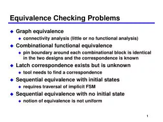
Outline Introduction BDDs The Davis-Putnam (DP) Procedure Equivalence Checking BDD-DP Relation Characteristics of CNF Formulas of Logic Circuits Relation between BDD and the DP Dynamic Variable Ordering for the DP Procedure Open questions Experimental Results Conclusions
Introduction BDDs have been traditionally used in logic synthesis and verification New Boolean satisfiability (SAT) solvers have shown recent promise as efficient equivalence checkers It is essential to understand the relation between BDDs and SAT procedures and show how the techniques of one domain can be applied to the other
x1 x2 x2 x3 x4 0 1 0 0 1 1 0 1 1 0 1 0 Binary Decision Diagrams ROBDDs are produced through the repeated application of Redundant test elimination Equivalent sub-graph sharing
a b d z 0 0 By unit clause propagation a d 0 By unit clause propagation z b c 0 1 The Davis-Putnam Procedure assign(sat_formula , literal v) begin a1. v = true; a2. simplify ; a3. apply unit clause propagation; a4. if has an empty clause then return false else return true; end DP(sat_formula ) begin d1. choose literal v to split on; d2. ifv = NULL then return true; d3. if assign(, v) then d4. if DP() then return true; d5. undo v assignment; d6. if assign(, v) then d7. if DP() then return true; d8. return false; end = (a + d) (b + d) (a + b + d) (c + z) (d + z) (d + c+ z). Consistent assignment achieved
c a d b d z z 1 1 By unit clause propagation a d 1 z b 1 By unit clause propagation c 1 1 The Davis-Putnam Procedure assign(sat_formula , literal v) begin a1. v = true; a2. simplify ; a3. apply unit clause propagation; a4. if has an empty clause then return false else return true; end DP(sat_formula ) begin d1. choose literal v to split on; d2. ifv = NULL then return true; d3. if assign(, v) then d4. if DP() then return true; d5. undo v assignment; d6. if assign(, v) then d7. if DP() then return true; d8. return false; end = (a + d) (b + d) (a + b + d) (c + z) (d + z) (d + c+ z). 0 0 0 0 1
Using BDDs Build the BDD of each circuit under verification and check that the BDDs are isomorphic Circuit I Using SAT Miter output Primary Input Check that the stuck-at-0 SAT formula of the miter circuit is unsatisfiable Circuit II Equivalence Checking Core equivalence checking techniques
A search in the decision trees of the two circuits for a path that leads to the terminal 1(0) in one but leads to the 0(1) terminal in the other. 1 0 Minimization of the number of paths to be compared Minimization of equivalence checking time Equivalence Checking Equivalence checking can be viewed as Decision tree of Circuit II Decision tree of Circuit I
Characteristics of CNF Formulas of Logic Circuits Let be a CNF formula generated from a logic circuit Let V() be the set of variables that depends on It is possible to find a set of variables P() V() such that can be satisfied by only splitting on the variables of P() in the DP procedure. P() is the set of primary inputs Reducing the number of decision variables introduces an overall reduction in the decision tree size
Let S denote the set of primary inputs currently assigned logic values under the assignment As If As is applied to , the resultant is the logic function fAs If v P() but v S then v is said to be redundant under As if fAs /v = 0 A CNF formula is satisfied under a truthassignment As of a set S P() if v(P()-S): fAs /v = 0 If the primary output variable is assigned a value under the current assignment then there is no point in further assignments Characteristics of CNF Formulas of Logic Circuits
1 a If S = {a} and Bs={a 1} then = (d) (b + d) (c + z) (d + z) (d + c+ z) Characteristics of CNF Formulas of Logic Circuits a d z b c = (a + d) (b + d) (a + b + d) (c + z) (d + z) (d + c+ z) = z P() = {a, b, c}
1 a If S = {a} and Bs={a 1} then = (d) (b + d) (c + z) (d + z) (d + c+ z) Under Bs fBs/b = 0 b is redundant Characteristics of CNF Formulas of Logic Circuits a d z b c = (a + d) (b + d) (a + b + d) (c + z) (d + z) (d + c+ z) = z P() = {a, b, c}
0 0 c If S = {c} and As={c 0} then z 0 and = (a + d) (b + d) (a + b + d). Characteristics of CNF Formulas of Logic Circuits a d z b c = (a + d) (b + d) (a + b + d) (c + z) (d + z) (d + c+ z) = z P() = {a, b, c}
0 0 c If S = {c} and As={c 0} then z 0 and = (a + d) (b + d) (a + b + d). Under Asboth fAs/a and fAs/b = 0 a & b are redundant Characteristics of CNF Formulas of Logic Circuits a d z b c = (a + d) (b + d) (a + b + d) (c + z) (d + z) (d + c+ z) = z P() = {a, b, c}
Characteristics of CNF Formulas of Logic Circuits Observation 1: DP decision space is reduced to be that of the primary inputs Observation 2: Redundant variables are not considered for decision in the DP procedure Observation 1 reduces the decision space to be like that of a BDD and observation 2 parallels the removal of redundant test in BDDs.
The equivalence checking problem between two circuits can be viewed as a search in the decision trees of the two circuits for a path that leads to the terminal 1(0) in one but leads to the 0(1) terminal in the other. 1 0 Decision tree of Circuit II Decision tree of Circuit I Relation between BDD and DP Given a BDD and a CNF formula for a logic circuit C, then under a variable ordering and a truth assignment Aon a certain path of to the terminal, is satisfiable using the same variable ordering and truth assignment.
x1 x2 x3 x4 x3 x2 x2 x1 x4 x2 9 paths in the BDD implies 8 backtracks in the CNF formula 0 1 0 1 Relation between BDD and DP BDD-DP Theorem For BDD with P paths and a CNF formula for a logic circuit C then if DP variable ordering strategy captures the same ordering for every path of ,then DP proves the equivalence of C against an equivalent version in P-1 backtracks. 0 1 0 1 0 0 0 0 1 1 1 1 0 0 1 1 1 1 0 0 Decision space of circuit I Decision space circuit II
Var_Choose() Assign a weight of 1.0 to the primary output For each circuit level from output to input: Divide the weight of the unbounded gate output among its inputs Accumulate the weight of the fan-out branches into the fan-out stem Return the PI with the largest weight Dynamic Variable Ordering for the DP Procedure DP dynamic variable ordering strategy should The variable ordering strategy should differ for every path of the decision tree No splitting on redundant variables Minimum number of splittings to reach the terminals
Assigns a weight of zero to redundant variables Tries to minimize the number of assignments to the terminals by splitting on the primary input with the largest weight The weights reflect structural properties of the circuit and should be considered as a heuristic to the optimal case Dynamic Variable Ordering for the DP Procedure The proposed dynamic variable ordering represent the structural impact of every primary input of the circuit
1/12 x1 1/4 1/4 i x2 1/12 1/2 j 1/4 f x3 1/2 1/2 h 1/3 x4 x3 Dynamic Variable Ordering for the DP Procedure 1
1/3 1/3 1/3 x3 x4 x2 x1 1 1 0 1 0 1 Dynamic Variable Ordering for the DP Procedure x1 1 i x2 1 j 1 f x3 h x4 1
For this example, the variable ordering that minimizes the number of BDD nodes (4) also minimizes the number of paths (6) In this case, the proposed dynamic variable ordering strategy faithfully captured the variable ordering of the minimum size BDD x3 x1 x2 x4 0 DP procedure proved the equivalence in an optimal number of 5 backtracks Dynamic Variable Ordering for the DP Procedure x1 i x2 j 1 f x3 1 h 1 x4 1 1 1 0 1 0 1
Questions that need answering I. Is there a relation between the number of nodes and the number of paths in a BDD? II. Does the minimum size BDD have the minimum number of paths? The first question remains an open problem After numerous experiments, we concluded that the minimum size BDD does not necessarily have the minimum number of paths BDD number of nodes and number of paths
Experimental Results The optimal is determined by picking the minimal path BDD resulting from sifting Average 90% reduction in the backtracks for the 21 functions of the ISCAS’89 benchmark circuits
Experimental Results Experiments carried out using a Pentime 233Mhz with 64 MB RAM Average 70% time reduction for the hard-SAT functions (13) of the ISCAS’ 89 benchmark circuits The multiplier c6288 number of paths does not significantly change for different variable orderings
Conclusions The relation between the search tree of the DP procedure and the BDD of the corresponding circuit was studied We established the relation between the number of paths in a BDD and the corresponding number of backtracks in the DP procedure, enabling the calculation of optimal lower bounds This relation enabled the inclusion of a modified BDD variable ordering heuristic in the splitting choice of the DP procedure Experimental results confirm the reported relation and demonstrate a dramatic decrease in the number of backtracks and time need to solve equivalence checking