Equivalence Checking Problems
Equivalence Checking Problems. Graph equivalence connectivity analysis (little or no functional analysis) Combinational functional equivalence pin boundary around each combinational block is identical in the two designs and the correspondence is known

Equivalence Checking Problems
E N D
Presentation Transcript
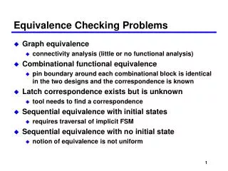
Equivalence Checking Problems • Graph equivalence • connectivity analysis (little or no functional analysis) • Combinational functional equivalence • pin boundary around each combinational block is identical in the two designs and the correspondence is known • Latch correspondence exists but is unknown • tool needs to find a correspondence • Sequential equivalence with initial states • requires traversal of implicit FSM • Sequential equivalence with no initial state • notion of equivalence is not uniform
Combinational Verification Algorithms • BDDs with decomposition points (Berman/Trevillyan ‘86) • ATPG (Automatic Test Pattern Generation) with decomposition points (Brand ‘93) • Recursive Learning (Kunz ‘93) • etc...
a 0 1 b b 0 1 0 1 c c c c 0 1 0 1 0 1 0 1 d d d d d d d d 0 0 0 1 0 0 0 1 0 0 0 1 1 1 1 1 Binary Decision Diagrams (Akers’78, Bryant’86) • Ordered decision tree for f = ab + cd
Subgraph reduction • Reduced Ordered Binary Decision Diagram (BDD) form: a 1 0 b 0 1 c 1 0 1 0 d 0 1 • Key idea: combine equivalent subcases
a c f f b BDD properties • Same order of variables on all paths • Reduced w.r.t. isomorphism • Variable ordering crucial for BDD size • Advantages: • canonical • trivial equivalence check • Disadvantages: • may be exponential in circuit size (especially multipliers) a 0 1 b 1 c 0 0 1 0 1 f = ac + abc a b c
Verification by monolithic BDDs =? • Single monolithic BDD for each output pair • BDD size may depend on variable ordering; some designs may have no efficient ordering
=? =? =? =? Verification by decomposed BDDs • How to generate good decomposition point pairs? • False negatives
Efficient false negative resolution is the key to equivalence checking on large combinational cones Say f1 = f2 If g1 is not equal to g2, then (f1 ||g1) may or may not be equal to (f2 ||g2) The false negative problem f1 g1 f1 ||g1 f2 g2 f2 ||g2
a b c d2 = b + cg + a c False negative example g = a b b d2 a d1 c d1 = bcg + (b + c) g Is [f = (d1 = d2)] equal to 1? f = d1 d2 + d1 d2 = b c + a g + b g + a b g Substitute value of g into f: f = b c + a (a b) + b (a b) + a b (a b) = 1
False negative resolution Is f(x1, x2, ..., xm, y1, y2, ... yk) = 1 ? where yi = gi(x1, x2, ..., xm, yi+1, ... yk) BDDs for • f(x1, x2, ..., xm, y1, y2, ... yk) • for each i, [yi = gi(x1, …, xm, yi+1, …, yk)] If f = 1 (false negative), decomposition points are equal, create a new decomposition point If f = 0 (real negative), we have a witness to prove that it is a real negative
Decomposition point selection • Tradeoff: • more decomposition points cause more false negative resolutions • fewer decomposition points cause larger sub-problems • Important to select more meaningful decomposition point candidates: • Separate primary input variables • Belong to the corresponding pairs of primary input cones
Candidates for decomposition points From design methodology: • pairs of nets with same or related names Through simulation: • First set by simulation of random/user-supplied vectors • Later simulations of witnesses of counterexamples for false negative resolution
Refining decomposition pairs by simulation a f h b x c g d i r e s i f x p x q g a p h b q c x s d r e
Refining decomposition pairs by simulation 0 a f 1 h b x c g 0 d i 1 r e s 1 i f x p x q 0 g a p h 1 b 0 q c x 1 s d r e 1
Refining decomposition pairs by simulation 0 a f 1 h b 0 x c g 0 0 0 d 1 i 1 r e 0 s 1 i f x p x q 0 g a p h 1 b 0 0 q c x 1 s d 1 r 0 e 0 0 1
Refining decomposition pairs by simulation 0 a f 1 h b 0 x c g 0 0 0 d 1 i 1 r e 0 s 1 i f x p x q 0 g a p h 1 b 0 0 q c x 1 s d 1 r 0 e 0 0 1
Refining decomposition pairs by simulation 1 a f 0 h b x c g 1 d i 0 r e s 0 i f x p x q 1 g a p h 0 b 1 q c x 0 s d r e 0
Refining decomposition pairs by simulation 1 a f 0 h b 0 x c g 0 1 1 d 1 i 0 r e 1 s 0 i f x p x q 1 g a p h 0 b 0 1 q c x 0 s d 1 r 1 e 1 1 0
Refining decomposition pairs by simulation 1 a f 0 h b 0 x c g 0 1 1 d 1 i 0 r e 1 s 0 i f x p x q 1 g a p h 0 b 0 1 q c x 0 s d 1 r 1 e 1 1 0
Refining decomposition pairs by simulation 1 a f 1 h b 1 x c g 1 0 1 d 1 i 1 r e 0 s 1 i f x p x q 1 g a p h 1 b 1 0 q c x 1 s d 1 r 1 e 0 0 1
Refining decomposition pairs by simulation 1 a f 1 h b 1 x c g 1 0 1 d 1 i 1 r e 0 s 1 i f x p x q 1 g a p h 1 b 1 0 q c x 1 s d 1 r 1 e 0 0 1
Candidates for decomposition points From design methodology: • pairs of nets with same or related names Through simulation: • First set by simulation of random/user-supplied vectors • Later simulations of witnesses of counterexamples for false negative resolution
c e Q 1 P f Candidates for decomposition points real negative witness simulation initial random simulation Real negatives can refine many other equivalence classes: c a e Q A P b e B c 1 P f Q f D d
False negative resolution example 1 a f 1 h b x c g 0 d i 0 r e 0 s i f x = = p =? x q 1 a p g h 1 b h = pqp = p = ab(c+d)= ab Counterexample: a=1 b=1 c=0 d=0 e=0 0 q c x 0 s d r e 0
False negative resolution example 1 a f 1 h b 1 x c g 0 0 0 d 0 i 0 r e 0 0 s i f x p x q 1 a p g h 1 b 1 0 q c x 0 s d 0 r 1 e 0 1 0
False negative resolution example 1 a f 1 h b 1 x c g 0 0 0 d 0 i 0 r e 0 0 s i f x p x q 1 a p g h 1 b 1 0 q c x 0 s d 0 r 1 e 0 1 0
False negative resolution - Solution 1 Is f(y1, y2, ... yk, x1, x2, ..., xm) = 1 ? where yi = gi(yi+1, ... yk, x1, x2, ..., xm) • Compose each decomposition point into f $ yi [f(y1, ... yk, x1, x2, ..., xm) (yi = gi(yi+1, ... yk, x2, ..., xm))] • Order of compositions is important • Stop if BDD = constant 1 or if there exists a path to 0-vertex consisting of only primary inputs Best when resulting BDD = constant 1 (false negative) [Intuition: final BDD is small (size = 1), so there might exist an order of compositions where no intermediate BDD blows up]
x5 y3 x2 Order of compositions f • Ordering heuristics: • compose yi so that the new support is minimized • compose yi such that the BDD for (yi = gi) is smallest • if yi is in support of both yj and f, compose yj • y1, y2, ... yk: have to compose each point at most once • Stop if BDD = constant 1 or if there exists a path to 0-vertex consisting of only primary inputs y1 y3 y2 y4 x1 x2 x3 x4 x5 0 1 1 0 0 1 0 1
False negative resolution - Solution 2 k+1 BDDs: f, (y1 = g1), …, (yk = gk) Find an assignment to all variables (y1, ... yk, x1, ..., xm) such that the corresponding path in each BDD leads to 1-vertex. If such an assignment exists, we have a witness for f = 0 (real negative); otherwise, f = 1 for all possible assignments (false negative) Search for an assignment among the set of all assignments. Works best if there exists one (or many) assignments (real negative).
Search strategies • Backtrack search: • pick an unassigned variable x • Set x=0, solve sub-problem • If fail, set x=1 and solve sub-problem • fail if any path in any BDD ends in 0-vertex, success if all paths end in 1-vertex • Local search: • pick a starting assignment to all variables • make a local move (flip a variable) so that cost function improves • success if all paths end in 1-vertex x4 0 1 x7 y1 0 1 1 y2 fail success 0 1 fail fail (x1 = 0, x2 = 1, y1 = 0) flip x2 x2 x1 y1 y1 y1 success
Summary of algorithm • Perform random simulation to obtain candidates for decomposition points • Verify decomposition point candidates: • if false negative, create a decomposition point • if real negative, refine future decomposition point candidates Heuristics for: • selecting a “good” subset of candidates • false negative resolution: “good” order of compositions or search for real negative • using real negatives to refine future candidates, to detect bugs early
ATPG with decomposition points (Brand’93) Stuck-at-1 fault redundancy => functional equivalence F X G X
Recursive Learning (Kunz’93) • Case analysis to learn implications between nets in the designs x2 = 1 g = 1 f = 1 x1 a d e b c f x2 g 1
Recursive Learning (Kunz’93) • Case analysis to learn implications between nets in the designs x2 = 1 g = 1 f = 1 x1 a d e b c f x2 1 g 1
Recursive Learning (Kunz’93) • Case analysis to learn implications between nets in the designs x2 = 1 g = 1 f = 1 x1 a d e b c b = 1 a = 1 f x2 1 g 1
Recursive Learning (Kunz’93) • Case analysis to learn implications between nets in the designs x2 = 1 g = 1 f = 1 1 x1 a d e b c b = 1 a = 1 f x2 1 g 1
Recursive Learning (Kunz’93) • Case analysis to learn implications between nets in the designs x2 = 1 0 g = 1 f = 1 1 x1 a d e b 1 c b = 1 a = 1 f x2 1 g 1 x1 = 1
Recursive Learning (Kunz’93) • Case analysis to learn implications between nets in the designs x2 = 1 g = 1 f = 1 x1 a d e 1 b c b = 1 a = 1 f x2 1 g 1 x1 = 1
Recursive Learning (Kunz’93) • Case analysis to learn implications between nets in the designs x2 = 1 0 g = 1 f = 1 x1 a d e 1 b 1 c b = 1 a = 1 f x2 1 g 1 x1 = 1 x1 = 1
Recursive Learning (Kunz’93) • Case analysis to learn implications between nets in the designs x2 = 1 g = 1 f = 1 x1 a d e b c b = 1 a = 1 f x2 g 1 x1 = 1 x1 = 1 1
Recursive Learning (Kunz’93) • Case analysis to learn implications between nets in the designs x2 = 1 g = 1 f = 1 x1 a d e b 1 0 0 c b = 1 a = 1 f x2 x1 = 1 g 1 x1 = 1 x1 = 1 1