Noise
Noise. Electromagnetic, Impulsive. A historically based tutorial by Robert J. Matheson Nov 14, 2013. Background:. The Nature of EM noise has changed over time, frequency, and technology.

Noise
E N D
Presentation Transcript
Noise Electromagnetic, Impulsive A historically based tutorial by Robert J. Matheson Nov 14, 2013
Background: The Nature of EM noise has changed over time, frequency, and technology. Some current questions about noise are partly historical. Therefore, a historical approach may help to enlighten the debate. Feel free to make comments or ask questions throughout the presentation
Speaker Intro: Robert J. Matheson –BA Physics, MS EE from CU 47 years at NTIA/ITS, retired 7 years ago. Began work in 1957 (summer job) with ARN-2 noise measurement program. Design of measurement system for ITS man-made noise program beginning in 1965. Radio Spectrum Measurement System program 1973-88, supporting NTIA frequency management. Deputy Director ITS Spectrum Division, 1988-91 ITS research – spectrum efficiency, property rights, technical spectrum policy, etc. 1991-2006
Topics 1951-65. ARN-2 worldwide measurements of lightning noise. 0-20 MHz. Impulsive noise, bandwidth effects, APDs, RMS, Vd, Ld. 1965-72. ITS Man-Made Noise program. .25-250 MHz. MMN sources, criteria, measurement techniques Recent MMN measurements. 2000-2013 Wider bandwidths, statistical processing. Future questions: What is noise? Where & How to measure?
ARN-2 Background: Atmospheric Radio Noise (ARN) measurements by NBS, 1956-65, at 8 frequencies (113 kHz – 20 MHz), 18 sites worldwide. Radio signals can be propagated (or not) around the world by multiple reflections off the ionosphere. Impulsive noise from lightning can also propagate worldwide, interfering with communications (60 dB change in average noise power). Received noise is dependent on global occurrence of thunderstorms and ionospheric propagation. Predicting hourly noise levels and noise statistics at any frequency and location is major goal.
ARN-2 Station ARN-2 Station: 4-m vertical whip antenna, surrounded by 100-ft diameter ground-plane. Frequencies: 113 kHz – 20 MHz
ARN-2 Receiver ARN-2 Noise Receiver 8 frequencies (113 kHz-20 MHz) RMS and Vd recorded on EA charts each hour.
Global ARN-2 NetworK ARN-2 Network: 16 stations operated by many nations 1956-1965. All personnel trained in Boulder, sites set up, EA chart records scaled and saved, equipment repaired in Boulder and returned to site.
ARN-2 Noise Maps World noise maps: 8 frequencies Four seasons in a year. Six 4-hr blocks in each day. 5-dB contour spacing CCIR Report 322 (1964) and future upgrades
ARN-2 Noise Maps ARN-2 Noise Program mission was largely completed with CCIR Report 322 in 1964. After “Cold War” ended, Russians and Chinese released compatible noise measurements and a revised report was created using the new data – NTIA TR-85-173. New radio technology has made these measurements less valuable. 1. Satellites, undersea optical fiber, higher radio frequencies have greatly eclipsed HF importance. 2. Automatic Link Establishment (ALE) continuously monitors several frequencies and chooses best.
Gaussian Noise (?) - - - - milliseconds - - - - Figure from Mark McHenry’s 2013 Powerline noise measurements – 2013. (67 MHz, 700 kHz BW) Noise Measurement ARN is impulsive noise produced by numerous, random (time and amplitude) lightning strokes. How can a bunch of random impulses be measured in a meaningful way?
Bandwidth = 2B 2V 0 T/2 Bandwidth = B/2 V/2 0 2xT Measuring EM impulses k Bandwidth = B Impulse = finite total energy infinite peak power zero time duration very wide uniform spectrum V 0 T
LARGER Bandwidth? Suppose the previous 700 kHz powerline noise were measured in a larger bandwidth? Perhaps 7 MHz BW (i.e., 10 x B) … • Bandwidth = 10 x B Add 20 dB to impulse amplitudes Add 10 dB to system noise • Note: 10 dB greater impulse-to-system noise ratio
Signal within 7 MHz measurement bandwidth? Larger Bandwidth?
Smaller Bandwidth? Suppose the previous 700-kHz powerline noise were measured in a smaller bandwidth? Perhaps 70 kHz BW (i.e., 0.1 x B)? • Bandwidth = 0.1 x B: Subtract 20 dB from impulses Subtract 10 dB from system noise • Note: 10 dB smaller impulse-to-SN ratio
Very small bandwidth? Suppose the previous powerline noise had been measured in a very small bandwidth? Perhaps 200 Hz ? (ARN-2) 4 kHz? (MMN) Pulses overlap, adding together in random phases, giving Gaussian-like noise. System noise or overlapping impulses? 8 impulses per msec
Various Bandwidths? Question: Which bandwidth gives the “right” answer to “show” the amount of noise? Answer: Wider BW impulses are higher, but possibly too fast (short duration) to see.
Choosing bandwidths How do you choose a measurement bandwidth? Choose bandwidth of prospective system, if known. Larger bandwidth data can be reduced to smaller BW easier than smaller BW can be changed to larger BW. Problems with larger bandwidth measurements: Need wider signal-free spectrum (signals contaminate noise measurements). Digitally excise signals? Larger bandwidth requires wider dynamic range and faster amplitude changes. Collect and process larger amounts of data if sampling based on X hours/min/sec to get statistical reliability.
Historic Bandwidths ARN-2 program: 200 Hz BW – dense signal environment over whole 0-20 MHz range. Used narrow guard-bands around WWV standard time signals (2.5, 5, 10, 20 MHz) + 13, 51, 160, 495 kHz. Limited dynamic range RMS detector (30-40 dB) ITS Man-Made Noise (MMN) measurements, 1965-75, .25-250 MHz, 4-kHz or 10-kHz BW, 60-dB RMS detector ITS 2001 MMN: 30 kHz, 2009 MMN: 1 MHz BW
In a typical frequency scan of narrowband signals, 10 x wider bandwidth raises system noise 10 dB, while signal amplitude remains same, hiding weaker signals below system noise. Also, 10 x wider bandwidth widens the spectral response, causing stronger signals to hide weaker signals. Therefore, wider measurement bandwidth generally hides in-formation on details of signal population, but improves details on impulsive noise populations. Signals vs bandwidth 195
Signals vs impulses: Note that measurement bandwidth typically affects signals and impulses in “opposite” ways. Impulsive noise: Increasing bandwidth increases the distance above internal system noise, makes more noise impulses appear. Signals: Increasing bandwidth decreases the distance above system noise for CW/modulated signals, signals overlap, makes fewer signals less visible.
Statistical noise data Question: How Can Statistical Noise Data Be Easily Summarized? Raw data - Highly detailed, but much more complex than for most needs. APDs (Amplitude probability distributions) - Good summary of amplitude statistics, but no time statistics. Various weighted averages – RMS - Average noise power/Hz - power per unit BW Vd – dB ratio between RMS and average voltage Ld – dB ratio between RMS and average log voltage Quasipeak – traditional, interference to AM voice
Statistical noise data Wepman, Figure 14. Noise time sample, 112.5 MHz, residential, 0349 AM.
Statistical noise data Summarizing data samples in APD or similar forms give an easy way to see impulsiveness of noise, detect low-level signals, identify independent noise sources, etc.
Statistical noise data Efficiently compute max, median, mean, min, RMS, Vd, Ld, etc. from APD instead of computing from individual data points. Efficiently compute levels that are exceeded certain percentages of time APD is an efficient form of data summary, representing possibly 100’s of millions of data points, but stored as 200-300 points
ITS Mobile noise APD APDs contain a stati-stical summary of data used to calcu-late various detector modes. Or, data can be proces-sed real-time by var-ious detectors and used to infer APDs. ARN, but less MMN Gaussian noise slope
ITS Mobile noise Lab 2-m vertical antenna Instrumentation And Crew Diesel generator Driver 1966 -1971 - ITS MMN measurement program.
ITS Mobile Noise LAB 1966-71
ITS Mobile noise lab Eight frequencies – 250 kHz to 250 MHz 4 kHz or 10 kHz Bandwidth RMS, Vd, Ld, Qd Sampled every 10 sec Vacuum tube receivers Transistor metering strips
ITS Mobile Noise Lab 8 receivers, 4 outputs digitized and recorded on digital mag tape every 10 sec. Mileage (0.01 mi res), time, and log event #. EA chart backup Optional printer output DM-2 gives 15-level APD for one channel.
ITS Mobile Noise Lab Typical operational configuration
ITS Mobile Noise Lab Three major measurement modes: Parked in various types of neighborhoods – residential, business, industrial, powerlines, highways, etc. Driving through traffic, to measure ignition noise in typical LMR environments. Multiple drives over fixed course to get average noise level contour maps of an area.
ITS Mobile noise APD 8 channels of RMS, Vd, Ld, Qd detectors. 1 channel of APD Correlate APD & dets so that detector read-ings provided likely APDs. Large dynamic range needed for various detectors. Gaussian noise slope
Noise contour map Geographical markers and mileage give location info. Multiple pass-es over fixed route gives data for noise contour map. Noise from base activities.
program: Following the 1965-1972 ITS MMN program, results were summarized by Spaulding “Man-Made Radio Noise – Part 1: Estimates for Business, Residential, and Rural Areas” NTIA Report OT-74-38. Measurements made occasionally to see if anything had changed significantly. Achatz & Dalke – “Man-made noise power measurements at VHF and UHF frequencies,” NTIA Report TR-02-390 Wepman – “Wideband man-made radio noise measurements in the VHF and low VHF bands,” NTIA Report TR-11-478. Decisions against need for larger noise program to thoroughly upgrade results.
24-hr noise data Wepman report “Wideband Man-made Radio Noise Measurements in the VHF and low UHF Bands,” NTIA Report TR-11-478 includes a number of 24-hr measurements at a number of different types of locations at 112 MHz, 220 MHz, and 401 MHz. Note: Previous extensive spectrum scans to find frequencies without signals. Some following examples …..
24-hr noise data Figure 19. Median, mean, and peak measured noise power in a 1-MHz bandwidth at a center frequency of 112.5 MHz at the Boulder residential location (August 31–September 1, 2009).
24-hr noise data Figure 20. Median, mean, and peak measured noise power in a 1-MHz bandwidth at a center frequency of 221.5 MHz at the Boulder residential location (September 3–4, 2009).
24-hr noise data Figure 21. Median, mean, and peak measured noise power in a 1-MHz bandwidth at a center frequency of 401 MHz at the Boulder residential location (September 2–3, 2009).
24-hr noise data Figure 22. Median, mean, and peak measured noise power in a 1-MHz bandwidth at a center frequency of 112.5 MHz at the Boulder business location (July 21–22, 2009).
24-hr noise data Figure 23. Median, mean, and peak measured noise power in a 1-MHz bandwidth at a center frequency of 221.5 MHz at the Boulder business location (July 20–21, 2009).
24-hr noise data Figure 29. Median, mean, and peak measured noise power in a 1-MHz bandwidth at a center frequency of 221.5 MHz at the Denver business location (August 18–19, 2009).
24-hr noise data Figure 34. Complementary cumulative distribution of the hourly median values of the median, mean, and peak powers in a 1-MHz bandwidth at a center frequency of approximately 112.5 MHz over both business locations.
program: The changing nature of noise: ARN : Noise is strictly impulsive, natural. Any man-made energy (signals or impulses) is rejected. MMN: Some ARN at lower frequencies (<20 MHz) cannot be avoided. MMN sources include powerlines, auto ignition, fluorescent lamps, electrical machinery, light dimmers, computers, switching power supplies, etc. Intentionally radiated (NB carrier) RF rejected/avoided. Note: Some noise looks like NB (dithered to widen). Today/tomorrow: Many “Gaussian noise-like” wideband signals, possible UWB impulse-like signals, many nonlicensed low-power, intermittent signals.
program: Where, when, how often to measure? ARN - 18 stations worldwide, 5 years. Very long range noise transmission, weather & solar cycles. MMN - Mobile radio used outdoors, highways. Noise measurements outdoors, highways. Today - Wireless, WiFi, nonlicensed used everywhere. Unlicensed low-powered signals play similar interfer-ence role as noise. Indoors, outdoors, vehicles, special events, office/business, houses, apartments, stores, malls, rooftops, trains, factories, power lines, rural, suburban, urban, etc. ID major sources?
program: What to do about noise-like signals? Measure everything, don’t try to discriminate. Extract/avoid known signals. Rest is “noise”. Use wider bandwidths to divide into “impulsive” noise and Gaussian floor (inc LP signals). This works until UWB. ITU-R Recommendation SM.1753-2 (2012) Methods for Measurements of Radio Noise. Intelligently excise known signal types; rest is noise. Et cetera …….???
THE END Questions? Comments? Robert Matheson November 14, 2013