Download
1 / 39
680 likes | 1.79k Vues
Chi-Squared Test of Homogeneity. Are different populations the same across some characteristic?. c 2 test for homogeneity. Used with a single categorical variable from two (or more) independent samples Used to see if the two populations are the same ( homogeneous )

E N D
Chi-Squared Test of Homogeneity Are different populations the same across some characteristic?
c2 test for homogeneity • Used with a single categorical variable from two (or more) independent samples • Used to see if the two populations are the same (homogeneous) • Several groups but STILL ONE VARIABLE
Assumptions & formula remain the same! • Samples are from a random sampling • All expected counts are greater than 5
Hypotheses – written in words H0: the proportions for the two (or more) distributions are the same Ha: At least one of the proportions for the distributions is different Be sure to write in context!
Assuming H0 is true, Expected Counts
Degrees of freedom Or cover up one row & one column & count the number of cells remaining!
Should Dentist Advertise? • It may seem hard to believe but until the 1970’s most professional organizations prohibited their members from advertising. In 1977, the U.S. Supreme Court ruled that prohibiting doctors and lawyers from advertising violated their free speech rights. • Why do you think professional organizations sought to prohibit their members from advertising?
Should Dentist Advertise? • The paper “Should Dentist Advertise?” (J. of Advertising Research (June 1982): 33 – 38) compared the attitudes of consumers and dentists toward the advertising of dental services. Separate samples of 101 consumers and 124 dentists were asked to respond to the following statement: “I favor the use of advertising by dentists to attract new patients.”
Should Dentist Advertise? • Possible responses were: strongly agree, agree, neutral, disagree, strongly disagree. • The authors were interested in determining whether the two groups—dentists and consumers—differed in their attitudes toward advertising.
Should Dentist Advertise? • This is a done by a chi-squared test of homogeneity, that is we are testing the claim that different populations have the same ratio across some second variable characteristic. • So how should we state the null and alternative hypotheses for this test?
Should Dentist Advertise? • H0: • Ha: The true category proportions for all responses are the same for both populations of consumers and dentists. The true category proportions for all responses are not the same for both populations of consumers and dentists.
Observed Data 101 124 • The expected cell counts are estimated from the sample data (assuming that H0 is true) by using … • How do we determine the expected cell count under the assumption of homogeneity?
Expected Values 101 124 19.30 • So the calculation for the first cell is …
Observed Data 14.36 14.36 22.89 19.30 30.08 17.64 28.11 23.70 36.92 17.64 • Students on the right side of the classroom finish the first row and the left side find the expected values for the dentists.
Conditions • So now we can consider the conditions of our analysis. • We will assume the data was randomly selected. • The sample was large enough because every cell in the contingency table had an expected frequency of at least 5.
Test Statistic • Now we can calculate the c 2 test statistic:
Sampling Distribution The two-way table for this situation has 2 rows and 5 columns, so the appropriate degrees of freedom is (2 – 1)(5 – 1) = 4. Since the likelihood of seeing such a large amount of difference between the observed frequencies and what we would expected to have seen if the two populations were homogeneous is so small (approx 0), there is strong evidence against the assumption that the proportions in the response categories are the same for the populations of consumers and dentists.
Post-graduation activities of graduates from an upstate NY high school Have what kids do after graduation changed across three graduating classes?
Could test whether two proportions are the same using a two-proportion z test…. but we have 3 groups. Chi-square goodness-of-fit tests against given proportions (theoretical models) …. but we want to know if choices have changed. So… we’ll use a chi-square test of homogeneity. Homogeneity means that things are the same so we have a built-in null hypothesis – the distribution does not change from group to group. This test looks for differences too large from what we might expect from random sample-to-sample variation.
Ho: The post-high school choices made by classes of 1980, 1990, 2000 have the same distributions Ha: The post-high school choices made by classes of 1980, 1990, 2000 do not have the same distributions Conditions: * categorical data with counts * expected values are all at least 5 Degrees of freedom: (R – 1)(C – 1) = 3 * 2 = 6 Test statistic:
= 72.77 P-value = P(x2 > 72.77) < 0.0001 The P-value is very small, so I reject the null hypothesis and conclude there is evidence that the choices made by high-school graduates have changed over the three classes examined.
When we reject the null hypothesis, it’s a good idea to examine residuals. To standardize the residuals: What can this show us?
The following data is on drinking behavior for independently chosen random samples of male and female students. Does there appear to be a gender difference with respect to drinking behavior? (Note: low = 1-7 drinks/wk, moderate = 8-24 drinks/wk, high = 25 or more drinks/wk)
Expected Counts: M F 0 158.6 167.4 L 554.0 585.0 M 230.1 243.0 H 38.4 40.6 • Assumptions: • Have 2 random sample of students • All expected counts are greater than 5. • H0: the proportions of drinking behaviors is the same for female & male studentsHa: at least one of the proportions ofdrinking behavior is different for female & male students • P-value = .000 df = 3 a = .05 • Since p-value < a, I reject H0. There is sufficient evidence to suggest that drinking behavior is not the same for female & male students.
c2 test for Independence • Used with categorical, bivariate data from ONEsample • Used to see if the two categorical variables are associated (dependent) or not associated (independent) • One sample but two variables
Hypotheses – written in words H0: two variables are independent Ha: two variables are dependent Be sure to write in context!
Assumptions & formula remain the same! Expected counts & df are found the same way as test for homogeneity. Only change is the hypotheses!
A study from the University of Texas Southwestern Medical Center examined whether the risk of hepatitis C was related to whether people had tattoos and to where they got their tattoos. Data differs from other kinds because they categorize subjects from a single group on two categorical variable rather than on only one.
Is the chance of having hepatitis C independent of tattoo status? If hepatitis status is independent of tattoos, we expect the proportion of people testing positive for hepatitis to be the same for the three levels of tattoo status. Are the categorical variables tattoo status and hepatitis statistically independent? A chi-square test for independence
Ho: Tattoo status and hepatitis status are independent Ha: Tattoo status and hepatitis status are not independent Conditions: * categorical data with counts * expected values are all at least 5 Degrees of freedom: (R – 1)(C – 1) = 2 * 1 = 2 Test statistic:
= 57.91 P-value = P(x2 > 57.91) < 0.0001
The p-value is very small, so I reject the null hypothesis and conclude that hepatitis status is not independent of tattoo status. Because the expected cell frequency condition was violated, I need to check that the two cells with small expected counts did not influence this result too greatly.
Whenever we reject the null hypothesis, it’s a good idea to examine the residuals. Since counts may be different for cells, we are better off standardizing the residuals. To standardize a cell’s residuals, divide by the square root of its expected value. The + and the – sign indicate whether we observed more cases than we expected, or fewer.
Examining the residuals: largest component: Hepatitis C/Tattoo parlor – suggest that a principal source of infection may be tattoo parlors second largest component: Hepatitis C/no tattoo – those who have no tattoos are less likely to be infected with hepatitis C than we might expect if the two variables are independent
A beef distributor wishes to determine whether there is a relationship between geographic region and cut of meat preferred. If there is no relationship, we will say that beef preference is independent of geographic region. Suppose that, in a random sample of 500 customers, 300 are from the North and 200 from the South. Also, 150 prefer cut A, 275 prefer cut B, and 75 prefer cut C.
If beef preference is independent of geographic region, how would we expect this table to be filled in? 90 60 165 110 45 30
Now suppose that in the actual sample of 500 consumers the observed numbers were as follows: (on your paper) Is there sufficient evidence to suggest that geographic regions and beef preference are not independent? (Is there a difference between the expected and observed counts?)
Assumptions: • Have a random sample of people • All expected counts are greater than 5. • H0: geographic region and beef preference are independentHa: geographic region and beef preference are dependent • P-value = .0226 df = 2 a = .05 • Since p-value < a, I reject H0. There is sufficient evidence to suggest that geographic region and beef preference are dependent. Expected Counts: N S A 90 60 B 165 110 C 45 30