Linear Programming
Linear Programming. Piyush Kumar (For Class of Dr. Ashok Srinivasan). Welcome to CIS5930-09. Optimization. For example. This is what is known as a standard linear program. Linear Programming. Significance A lot of problems can be converted to LP formulation

Linear Programming
E N D
Presentation Transcript
Linear Programming Piyush Kumar (For Class of Dr. Ashok Srinivasan) Welcome to CIS5930-09
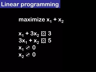
For example This is what is known as a standard linear program.
Linear Programming • Significance • A lot of problems can be converted to LP formulation • Perceptrons (learning), Shortest path, max flow, MST, matching, … • Accounts for major proportion of all scientific computations • Helps in finding quick and dirty solutions to NP-hard optimization problems • Both optimal (B&B) and approximate (rounding)
Graphing 2-Dimensional LPs Optimal Solution y Example 1: 4 Maximize x + y 3 x + 2 y ³ 2 Subject to: Feasible Region x £ 3 2 y £ 4 1 x ³0y ³0 0 x 0 1 2 3 These LP animations were created by Keely Crowston.
Graphing 2-Dimensional LPs Multiple Optimal Solutions! y Example 2: 4 Minimize ** x - y 3 1/3 x + y £ 4 Subject to: -2 x + 2 y £ 4 2 Feasible Region x £ 3 1 x ³0y ³0 0 x 0 1 2 3
Graphing 2-Dimensional LPs y Example 3: 40 Minimize x + 1/3 y 30 x + y ³ 20 Subject to: Feasible Region -2 x + 5 y £ 150 20 x ³ 5 10 x ³ 0y ³ 0 x 0 Optimal Solution 40 0 10 20 30
Do We Notice Anything From These 3 Examples? Extreme point y y y 4 40 4 3 3 30 2 2 20 1 1 10 0 0 0 x x x 0 1 0 1 2 0 10 20 2 3 3 30 40
A Fundamental Point y y y 4 40 4 3 3 30 2 2 20 1 1 10 0 0 0 x x x 0 1 0 1 2 0 10 20 2 3 3 30 40 If an optimal solution exists, there is always a corner point optimal solution!
Graphing 2-Dimensional LPs Optimal Solution Second Corner pt. y Example 1: 4 Maximize x + y 3 x + 2 y ³ 2 Subject to: Feasible Region x £ 3 2 y £ 4 1 x ³ 0y ³ 0 Initial Corner pt. 0 x 0 1 2 3
Then How Might We Solve an LP? • The constraints of an LP give rise to a geometrical shape - we call it a polyhedron. • If we can determine all the corner points of the polyhedron, then we can calculate the objective value at these points and take the best one as our optimal solution. • The Simplex Method intelligently moves from corner to corner until it can prove that it has found the optimal solution.
But an Integer Program is Different y • Feasible region is a set of discrete points. • Can’t be assured a corner point solution. • There are no “efficient” ways to solve an IP. • Solving it as an LP provides a relaxation and a bound on the solution. 4 3 2 1 0 x 0 1 2 3
Linear Programs in higher dimensions minimize z = 7x1 + x2 + 5x3 subject to x1 - x2 + 3x3 >= 10 5x1 + 2x2 - x3 >= 6 x1, x2, x3 0 What happens at (1,2,3)? What does it tell us about z* = optimal value of z?
LP Upper bounds • Any feasible solution to LP gives an upper bound on z* • So now we know z*<= 30. • How do we construct a lower bound? • z*>= 16? [Y/N]?
Lower bounding an LP • 7x1+x2+5x3 >= (x1-x2+3x3) + (5x1+2x2-x3) >= 16 • Find suitable multipliers ( >0 ?) to construct lower bounds. • How do we choose the multipliers?
The Dual maximize z’ = 10y1 + 6y2 subject to y1 + 5y2 <= 7 -y1 + 2y2 <= 1 3y1 – y2 <= 5 y1, y2 0 What is the dual of a dual? Every feasible solution of the dual gives a lower bound on z*
The Primal minimize z = 7x1 + x2 + 5x3 subject to x1 - x2 + 3x3 >= 10 5x1 + 2x2 - x3 >= 6 x1, x2, x3 0 Every feasible solution of the primal is an upper bound on the solution to the dual.
Primal – Dual picture Strong Optimality Primal = Dual at opt Z* 0 Primal Solutions Dual Solutions
Duality • A variable in the dual is paired with a constraint in the primal • Objective function of the dual is determined by the right hand side of the primal constraints • The constraint matrix of the dual is the transpose of the constraint matrix in the primal.
Duality Properties Some relationships between the primal and dual problems: • If one problem has feasible solutions and a bounded objective function (and so has an optimal solution), then so does the other problem, so both the weak and the strong duality properties are applicable • If the optimal value of the primal is unbounded then the dual is infeasible. • If the optimal value of the dual is unbounded then the primal is infeasible.
LP Geometry • Forms a n dimensional polyhedron • Is convex : If z1 and z2 are two feasible solutions then λz1+ (1- λ)z2 is also feasible. • Extreme points can not be written as a convex combination of two feasible points.
LP Geometry • The normals to the halfspaces defining the polyhedron are formed by the coefficents of the constraints. • Rows of A form the normals to the hyperplanes defining the primal LP pointing inside the polyhedron.
LP Geometry • Extreme point theorem: If there exists an optimal solution to an LP Problem, then there exists one extreme point where the optimum is achieved. • Local optimum = Global Optimum
LP: Algorithms • Simplex. (Dantzig 1947) • Developed shortly after WWII in response to logistical problems:used for 1948 Berlin airlift. • Practical solution method that moves from one extreme point to a neighboring extreme point. • Finite (exponential) complexity, but no polynomial implementation known. Courtesy Kevin Wayne
LP: Polynomial Algorithms • Ellipsoid. (Khachian 1979, 1980) • Solvable in polynomial time: O(n4 L) bit operations. • n = # variables • L = # bits in input • Theoretical tour de force. • Not remotely practical. • Karmarkar's algorithm. (Karmarkar 1984) • O(n3.5 L). • Polynomial and reasonably efficientimplementations possible. • Interior point algorithms. • O(n3 L). • Competitive with simplex! • Dominates on simplex for large problems. • Extends to even more general problems.
Ellipsoid Method Courtesy S. Boyd
Barrier central path • Predictor • Corrector Barrier Algorithms Simplex solution path Optimum Interior Point Methods
Complementary solutions • For any primal feasible (but suboptimal) x, its complementary solution y is dual infeasible, with cx=yb • For any primal optimal x*, its complementary solution y* is dual optimal, with cx*=y*b=z* • Duality Gap = cx-yb
Complementary slackness • x*, y* are simultaneously optimal for (P) and (D) iff • x* is opt for (P) and y* is opt for (D) OR • For I = 1..m if yi* > 0 • Then aix* = bi • For J = 1..n if xj* > 0 • Then y*Aj = ci ai are rows of A and Aj are the columns of A
Complementary slackness • x*, y* are simultaneously optimal for (P) and (D) iff • x* is opt for (P) and y* is opt for (D) OR • y*(Ax* - b) = 0 • (y*A – c)x* = 0 Summary: If a variable is positive, its dual constraint is tight Or if a constraint is loose its dual variable is zero.
Complementary Slackness • Proof? • y*(Ax* - b) - (y*A – c)x* = y*Ax* - y*b - y*Ax* + cx* = cx* - y*b = 0 ( But all terms are non-negative ) Hence all must be zero!
Algorithm Design Techniques • LP Relaxation • Rounding • Round the fractional solution obtained by solving LP-relaxation. • Runs fast • Primal Dual Schema • (iteratively constructs primal n dual solutions)
LP optimum y objective feasible solutions x Linear Program
optimum of LP relaxation IP optimum rounding down optimum of LP relaxation y objective feasible solutions = x Integer Program
Linear Relaxations • What happens if the optimal of a LP-Relaxation is Integral? • There are a class of IPs for which this is guaranteed to happen • Transportation problems • MaxFlow problems • In general (Unimodularity) … Exact Relaxation
Lower Bounds • Assume minimization problem • Any relaxation of the original IP has a _____________ optimal objective function value than the optimal objective function value of the original IP z*relaxation z* • z*relaxation is called a __________________ on z* • Difference between these two values is called the relaxation gap
Upper Bounds • Any feasible solution to the original IP has a _____________ objective function value than the optimal objective function value of the original IP zfeasible z* • zfeasible is called an __________________ on z* • Heuristic techniques can be used to find “good” feasible solutions • Efficient, may be beneficial if optimality can be sacrificed • Usually application- or problem-specific

