Maximum likelihood block method for denoising gamma-ray light curve
210 likes | 422 Vues
Maximum likelihood block method for denoising gamma-ray light curve. Collaboration Meeting Moscow, 6-10 Jun 2011. Agustín Sánchez Losa IFIC (CSIC – Universitat de València ). Outline. Flare Analysis Maximum Likelihood Blocks Likelihood Algorithms Brute force 1 Change Point

Maximum likelihood block method for denoising gamma-ray light curve
E N D
Presentation Transcript
Maximum likelihood block method for denoising gamma-ray light curve Collaboration Meeting Moscow, 6-10 Jun 2011 Agustín Sánchez Losa IFIC (CSIC – Universitat de València)
Outline • Flare Analysis • Maximum Likelihood Blocks • Likelihood • Algorithms • Brute force • 1 Change Point • 2 Change Point • Stop criteria • Likelihood threshold • Prior study • Fixed Prior • To-Do List Agustín Sánchez Losa – MoscowCollaboration Meeting
Flare Analysis • Find coincidences of gamma flares with neutrino events in ANTARES • Correlation proportional to the intensity of source’s flare light • Flare periods and intensities have to be identified by denoising the light curves. • Use of light curves measured by satellites (FERMI, SWIFT,...) Agustín Sánchez Losa – MoscowCollaboration Meeting
Flare Analysis • Different methods already described and used in the literature: • “Studies in astronomical time series analysis V” • Scargle J D 1998ApJ601, 151 • “IceCube: Multiwavelength search for neutrinos from transient point sources” • Resconi E 2007 J. Phys.: Conf. Ser. 60 223 • “On the classification of flaring states of blazars” • Resconi E 2009 arXiv:0904.1371v1 • “Studies in astronomical time series analysis VI” • Scargle’s Draft(2006) at his web page: “http://astrophysics.arc.nasa.gov/~jeffrey/” • Etcetera. • Scargle’s Draft describe a general method for different data types and some clues in the way to stop the algorithm • Finally studied method is the one for binned data perturbed by a known Gaussian error Agustín Sánchez Losa – MoscowCollaboration Meeting
Maximum Likelihood Blocks • General idea: • Data available (light curves): {xn,σn,tn} → {flux,error,time} • Divide the data in significant blocks of approximately constant rate in light emission, chosen and guided by a proper likelihood function • Flare duration irrelevant: not sensitive to the time value or gaps but the consecutive order of the flux values and their error • Algorithm: • Divide the data interval from only one block until N blocks (where N is the number of total data points) • Do it in an order that, every time the number of blocks is increased, try to represent qualitatively the different rate periods as best as possible (chosen likelihood) • Decide when to stop Agustín Sánchez Losa – MoscowCollaboration Meeting
Maximum Likelihood Blocks The first cell of a block define a Change Point (CP) Each cell represent a {xn,σn,tn} data A group of cells conform a block Every time the number of blocks is increased look, with a likelihood, for the cells in which is the most probable changes in the flux rate,considered constant inside the block, i.e. look for the most optimum CPs Another block Another CP Agustín Sánchez Losa – MoscowCollaboration Meeting
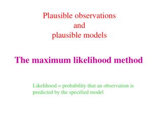
Maximum Likelihood Blocks • The likelihood for each block k, assuming that data, n, in that block comes from a constant rate λ perturbed by a Gaussian error, is: • The constant rate λ that maximize that likelihood is: • The total logarithmic likelihood, dropping the constant terms that are going to contribute always the same amount, is: Agustín Sánchez Losa – MoscowCollaboration Meeting
Maximum Likelihood Blocks • The remaining free parameters are the beginning of each block, or CPs (change points), and the total number of blocks, M, i.e. the total amount of CPs • The likelihood maximize with so many blocks as the total amount of data, i.e. a block or a CP for each data point, M = N • Once this is done remains the choice of the number of blocks to use, M Agustín Sánchez Losa – MoscowCollaboration Meeting
Algorithm • Brute force: try all possible CPs in the data, and chose the ones that maximize the likelihood. Too expensive in computing time. • One CP per iteration: in every step is maintained all the previously found CPs as the optimum ones and only a new CP is added, the one who maximize the likelihood. The best in time computing possible, and not a bad approximation at all, but some flares are more difficult to be found. • Two CPs per iteration: in every step “the 2 best CPs inside each block” are compared and chosen the pair which maximize the likelihood. Shows better capacity to detect evident flares in less number of blocks, M. 1CP 2CP Agustín Sánchez Losa – MoscowCollaboration Meeting
One CP testing... Likelihood 1CP 1-Log(L)/Log(Lmax) 1CP Number of blocks 130days Sampleforthe FERMI source 3C454.3 Agustín Sánchez Losa – MoscowCollaboration Meeting
One CP testing... Likelihood 1CP 1-Log(L)/Log(Lmax) 1CP “found-a-flare-gap” Number of blocks 50 days Sampleforthe FERMI source PMNJ2345-1555 Agustín Sánchez Losa – MoscowCollaboration Meeting
Two CP testing... Likelihood 2CP 1-Log(L)/Log(Lmax) 2CP Number of blocks 130days Sampleforthe FERMI source 3C454.3 Agustín Sánchez Losa – MoscowCollaboration Meeting
Two CP testing... Likelihood 2CP 1-Log(L)/Log(Lmax) 2CP Number of blocks 50 days Sampleforthe FERMI source PMNJ2345-1555 Agustín Sánchez Losa – MoscowCollaboration Meeting
Two CP testing... 2CP 300 days Small sampleforthe FERMI source 3C454.3 Agustín Sánchez Losa – MoscowCollaboration Meeting
Two CP testing... 2CP 300 days Small sampleforthe FERMI source 3C454.3 Agustín Sánchez Losa – MoscowCollaboration Meeting
Stop criteria • The chosen algorithm determine the order in which the CPs are added • The choice of when stop have been studied for the “Two CP per iteration” algorithm: • Likelihood threshold or similar: Stop when the likelihood value is a given percentage of the maximum likelihood. Not really useful criterion due to the different evolution of the likelihoods. • Scargle’s Prior Study: Made a study of the most optimum γfor this prior: to add to the logarithm likelihood in order to create a maximum. Pretty complicated and does not work with “flat-flared” light curves. • Fixed Scargle’s Prior: In the Scargle’s Draft is mentioned that γ should yields γ≈N, and that has been observed in the previous stop criterion. With this fixed value all flares are now detected but implies a bigger number of unnecessary blocks for the “easy-flares” light curves. Agustín Sánchez Losa – MoscowCollaboration Meeting
Stop criteria 1-Log(L)/Log(Lmax) • The chosen algorithm determine the order in which the CPs are added • The choice of when stop have been studied for the “Two CP per iteration” algorithm: • Likelihood threshold or similar: Stop when the likelihood value is a given percentage of the maximum likelihood. Not really useful criterion due to the different evolution of the likelihoods. • Scargle’s Prior Study: Made a study of the most optimum γfor this prior: to add to the logarithm likelihood in order to create a maximum. Pretty complicated and does not work with “flat-flared” light curves. • Fixed Scargle’s Prior: In the Scargle’s Draft is mentioned that γ should yields γ≈N, and that has been observed in the previous stop criterion. With this fixed value all flares are now detected but implies a bigger number of unnecessary blocks for the “easy-flares” light curves. 0208-512 3C454.3 Number of blocks 1-Log(L)/Log(Lmax) Number of blocks Agustín Sánchez Losa – MoscowCollaboration Meeting
Stop criteria Simulation of the light curve • The chosen algorithm determine the order in which the CPs are added • The choice of when stop have been studied for the “Two CP per iteration” algorithm: • Likelihood threshold or similar: Stop when the likelihood value is a given percentage of the maximum likelihood. Not really useful criterion due to the different evolution of the likelihoods. • Scargle’s Prior Study: Made a study of the most optimum γfor this prior: to add to the logarithm likelihood in order to create a maximum. Pretty complicated and does not work with “flat-flared” light curves. • Fixed Scargle’s Prior: In the Scargle’s Draft is mentioned that γ should yields γ≈N, and that has been observed in the previous stop criterion. With this fixed value all flares are now detected but implies a bigger number of unnecessary blocks for the “easy-flares” light curves. Application of thealgorithm Withdifferentγvaluesdifferentoptimum blocks forthesamples and different error between real light curve and obtained blocks Withdifferentγvaluesdifferentoptimum blocks forthesamples and different error between real light curve and obtained blocks Agustín Sánchez Losa – MoscowCollaboration Meeting
Stop criteria • The chosen algorithm determine the order in which the CPs are added • The choice of when stop have been studied for the “Two CP per iteration” algorithm: • Likelihood threshold or similar: Stop when the likelihood value is a given percentage of the maximum likelihood. Not really useful criterion due to the different evolution of the likelihoods. • Scargle’s Prior Study: Made a study of the most optimum γfor this prior: to add to the logarithm likelihood in order to create a maximum. Pretty complicated and does not work with “flat-flared” light curves. • Fixed Scargle’s Prior: In the Scargle’s Draft is mentioned that γ should yields γ≈N, and that has been observed in the previous stop criterion. With this fixed value all flares are now detected but implies a bigger number of unnecessary blocks for the “easy-flares” light curves. 40 days 70 days 100 days 1000 days Agustín Sánchez Losa – MoscowCollaboration Meeting
To Do List • Develop a base line estimator in order to define the flare period and build time PDFs • Start real data analyzing with those time PDFs Agustín Sánchez Losa – MoscowCollaboration Meeting
Thankyou foryourattention