Download
1 / 33
370 likes | 1.05k Vues
Power laws, Pareto distribution and Zipf's law. M. E. J. Newman Presented by: Abdulkareem Alali. Intro: Measurements distribution. One noticed observation on measuring quantities that they are scaled or centered around a typical value. As an example:

E N D
Power laws, Pareto distribution and Zipf's law M. E. J. Newman Presented by: Abdulkareem Alali
Intro: Measurements distribution One noticed observation on measuring quantities that they are scaled or centered around a typical value. As an example: • would be the heights of human beings. Most adult human beings are about 180cm tall. tallest and shortest adult men as having had heights 272cm and 57cm respectively, making the ratio 4.8. • another example of a quantity with a typical scale the speeds in miles per hour of cars on the motorway. Speeds are strongly peaked around 75mph.
Intro: Measurements distribution Another observation not all things we measure are peaked around a typical value. Some vary over an enormous dynamic range sometimes many orders of magnitude. As an example: The largest population of any city in the US is 8.00 million for New York City (2000). America’s smallest town is Duffield, Virginia, with a population of 52. the ratio of largest to smallest population is at least 150 000.
Intro: Measurements distribution America with a total population of 300 million people, you could at most have about 40 cities the size of New York. And the 2700 cities cannot have a mean population of more than 110,000. A histogram of city sizes plotted with logarithmic horizontal and vertical axes follows quite closely a straight line.
Intro: Measurements distribution Such histogram can be represented as ln(y) = A ln(x) + c Let p(x)dx be the fraction of cities with population between x and x + dx. If the histogram is a straight line on log-log scales, then ln(p(x)) = - ln(x) + c p(x) = C x−, C = ec
Intro: power low distribution This kind of distributionp(x) = C x− is called thepower low distribution. Power low implies that small occurrences are extremely common, whereas large instances are extremely rare.
Next: • Ways of detecting power-law behavior. • Give empirical evidence for power laws in a variety of systems.
Example on an artificially generated data set Take 1 million random numbers from a distribution with = 2.5 A normal histogram of the numbers, produced by binning them into bins of equal size 0.1. That is, the first bin goes from 1 to 1.1, the second from 1.1 to 1.2, and so forth. On the linear scales used this produces a nice smooth curve.
problem with Linear scale plot of straight bin of the data How many times did the number 1 or 3843 or 99723 occur, Power-law relationship not as apparent, Only makes sense to look at smallest bins first few bins whole range
I. Measuring Power Laws The author presents 3 ways to identifying power-law behavior: • Log-log plot • Logarithmic binning • Cumulative distribution function
10 20 30 100 200 1 2 3 1. Log-log plot Logarithmic axes : powers of a number will be uniformly spaced 20=1, 21=2, 22=4, 23=8, 24=16, 25=32, 26=64, ….
1. Log-log plot To fit power-law distributions the most common and not very accurate method: • Bin the different values of x and create a frequency histogram ln (# of times x occurred) ln(x)
problem with the Linear scale log-log plot of straight bin of the data the right-hand end of the distribution is noisy. Each bin only has a few samples in it, if any. So the fractional fluctuations in the bin counts are large and this appears as a noisy curve on the plot. here we have tens of thousands of observations when x < 10 Noise in the tail, less data in bins
Solution1:2. Logarithmic binning is to vary the width of the bins in the histogram. Normalizing the sample counts by the width of the bins they fall in. Number samples in a bin of width x should be divided by x to get a count per unit interval of x. The normalized sample count becomes independent of bin width on average. Most common choice is a fixed multiple wider bin than the one before it.
Logarithmic binning Example : Choose a multiplier of 2 and create bins that span the intervals 1 to 1.1, 1.1 to 1.3, 1.3 to 1.7 and so forth (i.e., the sizes of the bins are 0.1, 0.2, 0.4 and so forth). This means the bins in the tail of the distribution get more samples than they would if bin sizes were fixed. Bins appear more equally spaced. Logarithmic binning still have noise at the tail.
Solution2:3. Cumulative distribution function No loss of information • No need to bin, has value at each observed value of x. To have a cumulative distribution • i.e. how many of the values of x are at least x. • The cumulative probability of a power law probability distribution is also power law but with an exponent – 1.
Power laws, Pareto distribution and Zipf's law Cumulative distributions are sometimes also called rank/frequency. Cumulative distributions with a power-law form are sometimes said to follow Zipf’s law or a Pareto distribution, after two early researchers. “Zipf’s law” and “Pareto distribution” are effectively synonymous with “power-law distribution”. Zipf’s law and the Pareto distribution differ from one another in the way the cumulative distribution is plotted—Zipf made his plots with x on the horizontal axis and P(x) on the vertical one; Pareto did it the other way around. This causes much confusion in the literature, but the data depicted in the plots are of course identical.
Cumulative distributions vs. rank/frequency Sorting and ranking measurements and then plotting rank against those measurements is usually the quickest way to construct a plot of the cumulative distribution of a quantity. This the way the author used to plot all of the cumulative distributions in his paper.
Cumulative distributions vs. rank/frequency Plotting of the cumulative distribution function P(x) of the frequency with which words appear in a body of text: We start by making a list of all the words along with their frequency of occurrence. Now the cumulative distribution of the frequency is defined such that P(x) is the fraction of words with frequency greater than or equal to x (P(X x)). Alternatively one could simply plot the number of words with frequency greater than or equal to x.
Cumulative distributions vs. rank/frequency For example : The most frequent word, which is “the” in most written English texts. If x is the frequency with which this word occurs, then clearly there is exactly one word with frequency greater than or equal to x, since no other word is more frequent. Similarly, for the frequency of the second most common word—usually “of”—there are two words with that frequency or greater, namely “of” and “the”. And so forth. In other words, if we rank the words in order, then by definition there are n words with frequency greater than or equal to that of the nth most common word. Thus the cumulative distribution P(x) is simply proportional to the rank n of a word. This means that to make a plot of P(x) all we need do is sort the words in decreasing order of frequency, number them starting from 1, and then plot their ranks as a function of their frequency. Such a plot of rank against frequency was called by Zipf a rank/frequency plot.
Estimate from observed data One way is to fit the slope of the line in plots and this is the most commonly used method. For example, for the plot that was generated by Logarithmic binning gives = 2.26 ± 0.02, which is incompatible with the known value of = 2.5 from which the data were generated. An alternative, simple and reliable method for extracting the exponent is to employ the formula which gives = 2.500 ± 0.002 to the generated data.
Examples of power laws • Word frequency: Estoup. • Citations of scientific papers: Price. • Web hits: Adamic and Huberman • Copies of books sold. • Diameter of moon craters: Neukum & Ivanov. • Intensity of solar flares: Lu and Hamilton. • Intensity of wars: Small and Singer. • Wealth of the richest people. • Frequencies of family names: e.g. US & Japan not Korea. • Populations of cities.
The following graph is plotted using Cumulative distributions
Not everything is a power law • The abundance of North American bird species. • The number of entries in people’s email address • The distribution of the sizes of forest fires.
Conclusion The power-law statistical distributions seen in a wide variety of natural and man-made phenomena, from earthquakes and solar flares to populations of cities and sales of books. We have seen examples of power-law distributions in real data and seen 3 ways that have been used to measuring power laws.
References Power laws, Pareto distributions and Zipf’s law. M. E. J. Newman, Department of Physics and Center for the Study of Complex Systems, University of Michigan, Ann Arbor, MI 48109. U.S.A.