Download
1 / 24
240 likes | 274 Vues
Learn how to construct confidence intervals for means, proportions, differences, and design experiments with sample sizes. This comprehensive guide covers hypothesis testing, significance levels, p-values, and more.

E N D
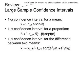
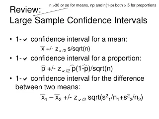
n >30 or so for means, np and n(1-p) both > 5 for proportions Review:Large Sample Confidence Intervals • 1-a confidence interval for a mean: x +/- za/2 s/sqrt(n) • 1-a confidence interval for a proportion: p +/- za/2 p(1-p)/sqrt(n) • 1-a confidence interval for the difference between two means: x1 – x2 +/- za/2 sqrt(s21/n1+s22/n2)
In General: ) ( Estimate (that is normally distributed via the CentralLimit Theorem) standard deviation Za/2of estimate +/- This gives an interval: (Lower Bound , Upper Bound) Interpretation: This is a plausible range for the true value of the number that we’re estimating. a is a tuning parameter for level of plausibility: smaller a = more conservative estimate.
np and n(1-p) > 5 for all p’s… Large Sample Confidence Intervals • 1-a confidence interval for difference between two proportions: p1-p2 +/- za/2 sqrt[(p1(1-p1)/n1)+(p2(1-p2)/n2)]
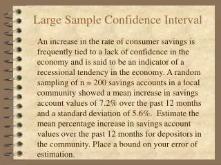
Designing an Experiment and Choosing a Sample Size • Example: Compare the shrinkage in a tumor due to a “new” cancer treatment relative to standard treatment • 100 patients randomly assigned to “new” treatment or standard treatment xinew = reduction in tumor size for person i under new treatment xjstd = reduction in tumor size for person j under std treatment xnew and s2new xstd and s2std Mean and sample variance of the changes in size for the new and standard treatments
Suppose the data are: xnew = 25.3 snew = 2.0 xstd = 24.8 sstd = 2.3 95% Confidence Interval for difference: x1 – x2 +/- za/2 sqrt(s21/n1+s22/n2) = 0.5 +/- 0.84 What can we conclude?
There’s no difference? • Can’t see a difference? • There’s a difference, but it’s too small to care about?
There is a difference between: • Can’t see a difference • There’s no difference Situation for Cancer example (In cancer experiment, we can assume we care about small differences.)
Can’t see a difference (that is big enough to care about) = wasted experiment • AVOID / PREVENT THE WASTE AND ASSOCIATED TEARS USE SAMPLE SIZE PLANNING
Sample Size Planning • Length of a 1-a level confidence interval is: “2 za/2 std deviation of estimate” 2za/2s/sqrt(n) 2za/2p(1-p)/sqrt(n) 2za/2sqrt((s21/n1)+(s22/n2)) 2za/2sqrt[(p1(1-p1)/n1)+(p2(1-p2)/n2)]
Suppose we want a 95% confidence interval no wider than W units. • a is fixed. Assume a value for the standard deviation (or variance) of the estimator. • Solve for an n (or n1 and n2) so that the width is less than W units. • When there are two sample sizes (n1 and n2), we often assume that n1 = n2.
Cancer example • Let W = 0.1. Want 95% CI for difference between means with width less than W. • Suppose s2new = s2std= 6 (conservative guess) W > 2za/2sqrt((s2new/n1)+(s2std/n2)) 0.1 > 2(1.96)sqrt(6/n + 6/n) 0.1 > 3.92sqrt(12/n) 0.01 > (3.922)12/n n > 18439.68 (each group…) Book’s B = our W/2
Hypothesis testing and p-values (Chapter 9) We used confidence intervals in two ways: • To determine an interval of plausible values for the quantity that we estimate. Level of plausibility is determined by 1-a. 90% (a=0.1) is less conservative than 95% (a=0.05) is less conservative than 99% (a=0.01)... • To see if a certain value is plausible in light of the data: If that value was not in the interval, it is not plausible (at certain level of confidence). Zero is a common certain value to test, but not the only one. Hypothesis tests address the second use directly
Example: Dietary Folate • Data from the Framingham Heart Study n = 333 Elderly Men Mean = x = 336.4 Std Dev = s = 193.4 Can we conclude that the mean is greater than 300 at 5% significance? (same as 95% confidence)
Five Components of the Hypothesis test: 1. Null Hypothesis = “What we want to disprove” = “H0” = “H not” = Mean dietary folate in the population represented by these data is <= 300. = m <= 300 2. Alternative Hypothesis = “What we want to prove” = “HA” = Mean dietary folate in the population represented by these data is > 300. = m > 300
3. Test Statistic To test about a mean with a large sample test, the statistic is z = (x – m)/(s/sqrt(n)) (i.e. How many standard deviations (of X) away from the hypothesized mean is the observed x?) 4. Significance Level of Test, Rejection Region, and P-value 5. Conclusion Reject H0 and conclude HA if test stat is in rejection region. Otherwise, “fail to reject” (not same as concluding H0 – can only cite a “lack of evidence” (think “innocent until proven guilty”) (Equivalently, reject H0 if p-value is less than a.) Next page
Significance Level: a=1% or 5% or 10%... (smaller is more conservative) (Significance = 1-Confidence) • Rejection Region: • Reject if test statistic in rejection region. • Rejection region is set by: • Assume H0 is true “at the boundary”. • Rejection region is set so that the probability of seeing the observed test statistic or something further from the null hypothesis is less than or equal to a • P-value • Assume H0 is true “at the boundary”. • P-value is the probability of seeing the observed test statistic or something further from the null hypothesis. • = “observed level of significance” Note that you reject if the p-value is less than a.(Small p-values mean “more observed significance”)
Example: • H0: m<=300, HA: m>300 • z (x-m)/(s/sqrt(n)) = (336.4 – 300)/(193.4/sqrt(333)) = 3.43 • Significance level = 0.05 • When H0 is true, Z~N(0,1). As a result, the cutoff is z0.05=1.645. (Pr(Z>1.645) = 0.05.) • P-value = Pr(Z>3.43 when true mean is 300) = 0.0003 • Reject. Mean is greater than 300. • Would you reject at significance level 0.0001?
Picture Distribution of Z = (X – 300)/(193.4/sqrt(333))when true mean is 300. Test statistic 0.4 0.3 Rejection region 0.2 Density Observed Test Statistic 0.1 0.0 -4 -2 0 2 4 3.43 1.645 Area to right of 3.43=0.0003 = p-value Test Statisistic Area to right of 1.645=0.05 = sig level
One Sided versus Two Sided Tests • Previous test was “one sided” since we’d only reject if the test statistic is far enough to “one side” (ie. If z > z0.05) • Two sided tests are more common (my opinion): H0: m=0, HA: m does not equal 0
Two Sided Tests (cntd) Test Statistic (large sample test of mean) z = (x – m)/(s/sqrt(n)) Rejection Region: reject H0 at signficance level a if |z|>za/2i.e. if z>za/2 or z<-za/2 Note that this “doubles” p-values. See next example.
Example: • H0: m=300, HA: m doesn’t equal 300 • z=(x-m)/(s/sqrt(n)) = (336.4 – 300)/(193.4/sqrt(333)) = 3.43 • Significance level = 0.05 • When H0 is true, Z~N(0,1). As a result, the cutoff is z0.025=1.96. (Pr(|Z|>1.96)=2*Pr(Z>1.96)=0.05 • P-value = Pr(|Z|>3.43 when true mean is 300) = Pr(Z>3.43) + Pr(Z<-3.43) = 2(0.0003)=0.0006 • Reject. Mean is not equal to 300. • Would you reject at significance level 0.0005?
Picture Distribution of Z = (X – 300)/(193.4/sqrt(333))when true mean is 300. Test statistic 0.4 Sig level = area to right of 1.96 + area to the left of -1.96 = 0.05=a 0.3 Rejection region Rejection region 0.2 Density 0.1 0.0 -4 -2 0 2 4 -3.43 3.43 1.96 1.96 Test Statisistic Area to right of 3.43=0.0003 Area to left of -3.43=0.0003 Pvalue=0.0006=Pr(|Z|>3.43)
Power and Type 1 and Type 2 Errors Action Fail to Reject H0 Reject H0 Significance level = a =Pr( Making type 1 error ) correct H0 True Type 1 error Truth Power = 1–Pr( Making type 2 error ) Type 2 error correct HA True
Assuming H0 is true, what’s the probability of making a type I error? • H0 is true means true mean is m0. • This means that the test statistic has a N(0,1) distribution. • Type I error means reject which means |test statistic| is greater than za/2. • This has probability a.