Interferometry in Radio Astronomy
660 likes | 1.04k Vues
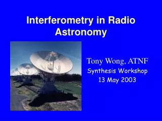
Interferometry in Radio Astronomy. Tony Wong, ATNF Synthesis Workshop 13 May 2003. Basic Concepts. An interferometer measures coherence in the electric field between pairs of points (baselines). Direction to source. wavefront. c t. Bsin . . B. T2. T1. (courtesy Ray Norris).

Interferometry in Radio Astronomy
E N D
Presentation Transcript
Interferometry in Radio Astronomy Tony Wong, ATNF Synthesis Workshop 13 May 2003
Basic Concepts • An interferometer measures coherence in the electric field between pairs of points (baselines). Direction to source wavefront ct Bsin B T2 T1 (courtesy Ray Norris) Correlator • Because of the geometric path difference ct, the incoming wavefront arrives at each antenna at a different phase.
Basic Concepts Young’s double slit experiment: constructive interference occurs when path difference is an integer number of wavelengths. from Dave McConnell
Basic Concepts • Consider a 2-element east-west interferometer. • By analogy to the double slit experiment, regions which would cause constructive and destructive interference can be considered “stripes” in the sky. west meridian east
l/(2B) radians Basic Concepts The angular resolution of the interferometer is given by the fringe half-spacing l/(2B). west meridian east
Basic Concepts • As the source moves through the fringe pattern, it produces an oscillating output signal from the interferometer. west meridian east
output signal Basic Concepts • If the source is very small compared to the fringe half-spacing l/(2B), we say it is unresolved. The output signal is just the fringe pattern, and the source structure cannot be determined. west meridian east
Basic Concepts • If the source is comparable to the fringe half-spacing l/(2B), then the output signal is the fringe pattern smoothed by the finite size of the source. west meridian east
Basic Concepts • If the source is large enough to span both a peak and a trough in the fringe pattern, the output signal is nearly constant. The source is over-resolved or “resolved out”, and its structure poorly determined. west meridian east
Basic Concepts • If you are interested in source structure that is being resolved out, then observe with a shorter baseline B to make the fringe spacing l/B larger. west meridian east
Basic Concepts • The primary beam of each antenna has a diameter ~l/D, which is always larger than the fringe spacing because D<B. The primary beam gives the FOV. west meridian east
The 2nd Dimension With a single baseline it would appear that we only get information about the source structure in one dimension! How do we know it’s not like this?
The 2nd Dimension However, for circumpolar objects the source traces a circle with respect to the fringe pattern, so 2D info can be obtained, if you observe long enough. SCP
The 2nd Dimension For sources closer to the celestial equator, the path is less curved and one obtains little information on N-S structure (for a pure E-W array).
Bandwidth smearing • Since the fringe spacing is proportional to wavelength, different frequencies in the observing band will have slightly different fringe patterns. west meridian east 1420 MHz
Bandwidth smearing • Since the fringe spacing is proportional to wavelength, different frequencies in the observing band will have slightly different fringe patterns. west meridian east 1430 MHz
Bandwidth smearing • As a result, constructive interference (“coherence”) is only strictly maintained at the meridian, where the path lengths to the two telescopes are equal. west meridian east White light fringe
Phase centre ct B T2 T1 Correlator Delay tracking To counter this problem, a variable delay is added to the signal from one dish, causing the white light fringe to follow the source across the sky. Extra delay ct added in electronics for T2
structures here would be invisible! Delay tracking However, by having the fringes move with the source, less information is available about the source structure. Phase centre
Delay tracking So, a phase shift of p/2 is periodically inserted to effectively shift the fringe pattern (this is done automatically by using a complex correlator). Phase centre
Delay tracking So, a phase shift of p/2 is periodically inserted to effectively shift the fringe pattern (this is done automatically by using a complex correlator). Phase centre
Fringe rotation Delay tracking can also cause the fringes to rotate! Phase centre 00:00
Fringe rotation Delay tracking can also cause the fringes to rotate! 03:00
Fringe rotation Delay tracking can also cause the fringes to rotate! 06:00
Fringe rotation Delay tracking can also cause the fringes to rotate! 09:00
ct B T2 T1 Fringe rotation The basic reason is that by inserting additional delays, you are effectively moving one of the antennas closer or further from the source. Moving the baseline produces a change in the fringe pattern. 12:00
Getting Confusing? • Clearly, tracking a source across the sky provides a great deal more information than a “snapshot” observation, because the source is sampled with a variety of fringe spacings, which are at different angles to the source. • One way to formalise this is to adopt the “view” from the source, which sees the array rotating beneath it. • This leads to the concept of the visibility plane, and the powerful technique of aperture synthesis.
The Visibility Plane • The projection of a baseline onto the plane normal to the source direction defines a vector in (u,v) space, measured in wavelength units. (u,v)
Aperture Synthesis • As the source moves across the sky (due to Earth’s rotation), the baseline vector traces part of an ellipse in the (u,v) plane. B sin = (u2 + v2)1/2 v (kl) Bsin T2 u (kl) B T1 T2 T1 • Actually we obtain data at both (u,v) and (-u,-v) simultaneously, since the two antennas are interchangeable. Ellipse completed in 12h, not 24!
214m 31m Aperture Synthesis • Example: 5 moveable antennas of ATCA, in the EW214 configuration. north east 10 baselines ranging from 31m to 214m 9.1 to 63 kl at 88 GHz
Aperture Synthesis • Instantaneous (u,v) coverage near transit • 10 baselines, 20 (u,v) points
Aperture Synthesis • (u,v) coverage for full 12 hour observation at declination –80.
Aperture Synthesis • Simulated (u,v) coverage for a single dish telescope of diameter 200m.
Aperture Synthesis Hence the term “aperture synthesis”!
Visibility Function • The output of the interferometer, after multiplying each pair of signals, is the complex visibility, V =|V|ei, which has an amplitude and phase. • The Fourier transform of the complex visibility with respect to (u,v) gives the sky intensity distribution. Hence (u,v) = spatial frequencies.
FT Sampling of Visibility Plane • If the (u,v) plane is incompletely sampled, the point spread function (PSF) has artefacts (“sidelobes”). Point source response of 3 antennas (3 baselines)
FT Sampling of Visibility Plane • Adding one antenna to an N element array adds N-1 baselines! Imaging quality increases faster than linearly with array size. Point source response of 5 antennas (10 baselines)
Data Reduction After obtaining raw visibilities, the usual procedure is: • Calibration of visibilities using data from one or more bright point sources, observed at regular intervals during the observation. • Establish the flux density scale (Jy) using a standard source. • Inverse Fourier transform to make a “dirty map.” • Deconvolution to remove artefacts due to the PSF.
Högbom’s CLEAN algorithm • Locate the peak in the map. • Subtract off a scaled version of the PSF or “dirty beam.” • Repeat until only noise left in image. • Add back the subtracted components in the form of Gaussians (“clean beams”) with size comparable to the centre of the PSF.
Deconvolution Dirty map CLEANed map
Advantages of interferometers • Can achieve much higher angular resolution than single-dish telescopes. • Less affected by pointing errors: position of the phase tracking centre determined by the observatory clock, and is independent of the pointing of the individual antenna elements. • Less affected by gain fluctuations on an individual antenna, as long as they are uncorrelated with other antennas. Long integrations possible. • Spectral baselines usually flat for same reason. • Can adjust the resolution of the map by re-weighting the visibilities in software.
Centimetre Arrays Westerbork Synthesis Radio Telescope, Netherlands 14 antennas (4 moveable) x 25m diameter, 300 MHz – 9 GHz
Centimetre Arrays Very Large Array, Socorro NM USA 27 moveable antennas x 25m diameter, 73 MHz – 50 GHz
Centimetre Arrays Australia Telescope Compact Array, Narrabri NSW 6 antennas (5 moveable) x 22m diameter, 1 – 9 GHz (being upgraded to ~22 and ~100 GHz)
Centimetre Arrays Ryle Telescope, Cambridge, UK 8 antennas (4 moveable) x 13m diameter, 15 GHz
Centimetre Arrays Molongolo Observatory Synthesis Telescope, Canberra ACT 2 fixed cylindrical paraboloids 778m long, 843 MHz
Centimetre Arrays DRAO Synthesis Telescope, Penticton BC Canada 7 antennas (3 moveable) x 9m diameter, 408 & 1420 MHz
Centimetre Arrays Mauritius Radio Telescope, Mauritius 1088 helical antennas, 151 MHz
Centimetre Arrays Giant Metrewave Radio Telescope, Pune, India 30 fixed antennas x 45m diameter, 150 – 1420 MHz
Millimetre Arrays Plateau de Bure Interferometer, France 6 antennas x 15m diameter, 80 – 250 GHz