Inferences about Variances ( Chapter 7)
170 likes | 466 Vues
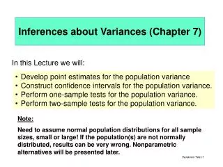
Inferences about Variances ( Chapter 7). In this Lecture we will:. Develop point estimates for the population variance Construct confidence intervals for the population variance. Perform one-sample tests for the population variance. Perform two-sample tests for the population variance.

Inferences about Variances ( Chapter 7)
E N D
Presentation Transcript
Inferences about Variances (Chapter 7) In this Lecture we will: • Develop point estimates for the population variance • Construct confidence intervals for the population variance. • Perform one-sample tests for the population variance. • Perform two-sample tests for the population variance. Note: Need to assume normal population distributions for all sample sizes, small or large! If the population(s) are not normally distributed, results can be very wrong. Nonparametric alternativeswill be presented later.
Point Estimate for 2 The point estimate for 2 is the sample variance: What about the sampling distribution of s2? (I.e. what would we see as a distribution for s2 from repeated samples). If the observations, yi, are from a normal (,) distribution, then the quantity has a Chi-square distribution with df = n-1.
Chi Square (2) Distribution Non-symmetric. Shape indexed by one parameter called the degrees of freedom (df).
Chi Square Table Table 7 in Ott and Longnecker
Confidence Interval for 2 12.83 20.48 .8312 3.247 df=5 df=10 .95 .95 has a Chi Square Distribution, then a 100(1-)% CI can be computed by finding the upper and lower /2 critical values from this distribution. If
Consider the data from the contaminated site vs. background. Background Data: A 95% CI for background population variance s2 = 1.277
Hypothesis Testing for s2 Test Statistic: Example: In testing Ha: 2 > 1: Reject H0 if 2 > 26,0.05 =12.59 Conclude: Do not reject H0. What if we were interested in testing: Rejection Region: 1. Reject H0 if 2 > 2df, 2. Reject H0 if 2 < 2df,1- 3. Reject H0 if either 2 < 2df,1-/2 or 2 > 2df,/2
Tests for Comparing Two Population Variances has a probability distribution in repeated sampling which follows the F distribution. F(2,5) The F distribution shape is defined by two parameters denoted the numerator degrees of freedom (ndf or df1 ) and the denominator degrees of freedom (ddf or df2 ). F(5,5) Objective: Test for the equality of variances (homogeneity assumption).
F distribution: • Can assume only positive values (like 2, unlike normal and t). • Is nonsymmetrical (like 2, unlike normal and t). • Many shapes -- shapes defined by numerator and denominator degrees of freedom. • Tail values for specific values of df1 and df2 given in Table 8. df1 relates to degrees of freedom associated with s21 df2 relates to degrees of freedom associated with s22
F Table Table 8 Numerator df = df1. Note this table has three things to specify in order to get the critical value. Denominator df = df2. 4.28 5.82 Probability Level
Hypothesis Test for two population variances Test Statistic: For one-tailed tests, define population 1 to be the one with larger hypothesized variance. Rejection Region: • Reject H0 if F > Fdf1,df2,. • Reject H0 if F > Fdf1,df2,/2 or if F < Fdf1,df2,1-/2. • In both cases, df1=n1-1 and df2=n2 -1. versus
Example Study Site Samples Background Samples T.S. R.R. Reject H0 if F > Fdf1,df2, where df1=n1-1 and df2=n2-1 = 0.05, F6,6,0.05 = 4.28 One-sided Alternative Hypothesis Reject H0 if F > Fdf1,df2,/2 or if F < F df1,df2,1-/2 = 0.05, F6,6,0.025 = 5.82, F6,6,0.975 = 0.17Two-sided Alternative Conclusion: Do not reject H0 in either case.
(1-)100% Confidence Interval for Ratio of Variances Example (95% CI): Note: not a argument! Note: degrees of freedom have been swapped.
Conclusion While the two sample test for variances looks simple (and is simple), it forms the foundation for hypothesis testing in Experimental Designs (ANOVA). • Nonparametric alternatives are: • Levene’s Test (Minitab); • Fligner-Killeen Test (R).
Software Commands for Chapters 5, 6 and 7 MINITAB Stat -> Basic Statistics -> 1-Sample z, 1-Sample t, 2-Sample t, Paired t, Variances, Normality Test. -> Power and Sample Size -> 1-Sample z, 1-Sample t, 2-Sample t. -> Nonparametrics -> Mann-Whitney (Wilcoxon Rank Sum Test) -> 1-sample Wilcoxon (Wilcox. Signed Rank Test) R t.test( ): 1-Sample t, 2-Sample t, Paired t. power.t.test( ): 1-Sample t, 2-Sample t, Paired t. var.test( ): Tests for homogeneity of variances in normal populations. wilcox.test( ): Nonparametric Wilcoxon Signed Rank & Rank Sum tests. shapiro.test( ), ks.test( ): tests of normality.
Example • It’s claimed that moderate exposure to ozone increases lung capacity. 24 similar rats were randomly divided into 2 groups of 12, and the 2nd group was exposed to ozone for 30 days. The lung capacity of all rats were measured after this time. • No-Ozone Group: 8.7,7.9,8.3,8.4,9.2,9.1,8.2,8.1,8.9,8.2,8.9,7.5 • Ozone Group: 9.4,9.8,9.9,10.3,8.9,8.8,9.8,8.2,9.4,9.9,12.2,9.3 • Basic Question: How to randomly select the rats? • In class I will demonstrate the use of MTB and R to analyze these data. (See “Comparing two populations via two sample t-tests” in my R resources webpage.)