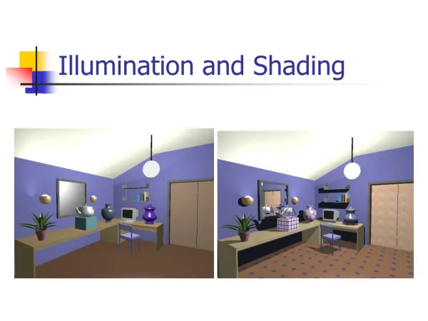
Illumination and Shading
Illumination and Shading. Light Sources Empirical Illumination Shading Transforming Normals . Illumination Models. Illumination The transport luminous flux from light sources between points via direct and indirect paths Lighting The process of computing the luminous

Illumination and Shading
E N D
Presentation Transcript
Illumination and Shading Light Sources Empirical Illumination Shading Transforming Normals
Illumination Models • Illumination • The transport luminous flux • from light sources between • points via direct and indirect paths • Lighting • The process of computing the luminous • intensity reflected from a specified 3-D point • Shading • The process of assigning a colors to a pixels • Illumination Models • Simple approximations of light transport • Physical models of light transport Slide 2
Two Components of Illumination • Light Sources (Emitters) • Emission Spectrum (color) • Geometry (position and direction) • Directional Attenuation • Surface Properties (Reflectors) • Reflectance Spectrum (color) • Geometry (position, orientation, and micro-structure) • Absorption • Approximations • Only direct illumination from the emitters to the reflectors • Ignore the geometry of light emitters, and consider only the geometry of reflectors Slide 3
Ambient Light Source • Even though an object in a scene is not directly lit it will still be visible. This is because light is reflected indirectly from nearby objects. A simple hack that is commonly used to model this indirect illumination is to use of an ambient light source. Ambient light has no spatial or directional characteristics. The amount of ambient light incident on each object is a constant for all surfaces in the scene. An ambient light can have a color. • The amount of ambient light that is reflected by an object is independent of the object's position or orientation. Surface properties are used to determine how much ambient light is reflected. Slide 4
Directional Light Sources • All of the rays from a directional light source have a common direction, and no point of origin. It is as if the light source was infinitely far away from the surface that it is illuminating. Sunlight is an example of an infinite light source. • The direction from a surface to a light source is important for computing the light reflected from the surface. With a directional light source this direction is a constant for every surface. A directional light source can be colored. Slide 5
Point Light Sources • The point light source emits rays in radial directions from its source. A point light source is a fair approximation to a local light source such as a light bulb. • The direction of the light to each point on a surface changes when a point light source is used. Thus, a normalized vector to the light emitter must be computed for each point that is illuminated. Slide 6
Other Light Sources • Spotlights • Point source whose intensity falls off away from a given direction • Requires a color, a point, a direction, parameters that control the rate of fall off • Area Light Sources • Light source occupies a 2-D area (usually a polygon or disk) • Generates soft shadows • Extended Light Sources • Spherical Light Source • Generates soft shadows Slide 7
Ideal Diffuse Reflection • First, we will consider a particular type of surface called an ideal diffuse reflector. An ideal diffuse surface is, at the microscopic level a very rough surface. Chalk is a good approximation to an ideal diffuse surface. Because of the microscopic variations in the surface, an incoming ray of light is equally likely to be reflected in any direction over the hemisphere. Slide 8
Lambert's Cosine Law • Ideal diffuse reflectors reflect light according to Lambert's cosine law, (there are sometimes called Lambertian reflectors). Lambert's law states that the reflected energy from a small surface area in a particular direction is proportional to cosine of the angle between that direction and the surface normal. Lambert's law determines how much of the incoming light energy is reflected. Remember that the amount energy that is reflected in any one direction is constant in this model. In other words the reflected intensity is independent of the viewing direction. The intensity does however depend on the light source's orientation relative to the surface, and it is this property that is governed by Lambert's law. Slide 9
Computing Diffuse Reflection • The angle between the surface normal and the incoming light ray is called the angle of incidence and we can express a intensity of the light in terms of this angle. • The Ilight term represents the intensity of the incoming light at the particular wavelength (the wavelength determines the light's color). The kd term represents the diffuse reflectivity of the surface at that wavelength. • In practice we use vector analysis to compute cosine term indirectly. If both the normal vector and the incoming light vector are normalized (unit length) then diffuse shading can be computed as follows: Slide 10
Diffuse Lighting Examples • We need only consider angles from 0 to 90 degrees. Greater angles (where the dot product is negative) are blocked by the surface, and the reflected energy is 0. Below are several examples of a spherical diffuse reflector with a varying lighting angles. • Why do you think spheres are used as examples when shading? Slide 11
Specular Reflection • A second surface type is called a specular reflector. When we look at a shiny surface, such as polished metal or a glossy car finish, we see a highlight, or bright spot. Where this bright spot appears on the surface is a function of where the surface is seen from. This type of reflectance is view dependent. • At the microscopic level a specular reflecting surface is very smooth, and usually these microscopic surface elements are oriented in the same direction as the surface itself. Specular reflection is merely the mirror reflection of the light source in a surface. Thus it should come as no surprise that it is viewer dependent, since if you stood in front of a mirror and placed your finger over the reflection of a light, you would expect that you could reposition your head to look around your finger and see the light again. An ideal mirror is a purely specular reflector. • In order to model specular reflection we need to understand the physics of reflection. Slide 12
Snell's Law • Reflection behaves according to Snell's law: • The incoming ray, the surface normal, and the reflected ray all lie in a common plane. • The angle that the reflected ray forms with the surface normal is determined by the angle that the incoming ray forms with the surface normal, and the relative speeds of light of the mediums in which the incident and reflected rays propagate according to the following expression. (Note: nl and nr are the indices of refraction) Slide 13
Reflection • Reflection is a very special case of Snell's Law where the incident light's medium and the reflected rays medium is the same. Thus we can simplify the expression to: Slide 14
Non-ideal Reflectors • Snell's law, however, applies only to ideal mirror reflectors. Real materials, other than mirrors and chrome tend to deviate significantly from ideal reflectors. At this point we will introduce an empirical model that is consistent with our experience, at least to a crude approximation. • In general, we expect most of the reflected light to travel in the direction of the ideal ray. However, because of microscopic surface variations we might expect some of the light to be reflected just slightly offset from the ideal reflected ray. As we move farther and farther, in the angular sense, from the reflected ray we expect to see less light reflected. Slide 15
Phong Illumination • One function that approximates this fall off is called the Phong Illumination model. This model has no physical basis, yet it is one of the most commonly used illumination models in computer graphics. • The cosine term is maximum when the surface is viewed from the mirror direction and falls off to 0 when viewed at 90 degrees away from it. The scalar nshiny controls the rate of this fall off. Slide 16
Effect of the nshiny coefficient • The diagram below shows the how the reflectance drops off in a Phong illumination model. For a large value of the nshiny coefficient, the reflectance decreases rapidly with increasing viewing angle. Slide 17
Computing Phong Illumination • The V vector is the unit vector in the direction of the viewer and the R vector is the mirror reflectance direction. The vector R can be computed from the incoming light direction and the surface normal: Slide 18
Blinn & Torrance Variation • Jim Blinn introduced another approach for computing Phong-like illumination based on the work of Ken Torrance. His illumination function uses the following equation: • In this equation the angle of specular dispersion is computed by how far the surface's normal is from a vector bisecting the incoming light direction and the viewing direction. • On your own you should consider • how this approach and the previous • one differ. Slide 19
Phong Examples • The following spheres illustrate specular reflections as the direction of the light source and the coefficient of shininess is varied. Slide 20
Putting it all together • Phong Illumination Model Slide 21
Phong Illumination Model • for each light Ii • for each color component • reflectance coefficients kd, ks, and kascalars between 0 and 1 may or may not vary with color • nshinyscalar integer: 1 for diffuse surface, 100 for metallic shiny surfaces • notice that the specular component does not depend on the object color . Slide 22
Where do we Illuminate? • To this point we have discussed how to compute an illumination model at a point on a surface. But, at which points on the surface is the illumination model applied? Where and how often it is applied has a noticeable effect on the result. • Illuminating can be a costly process involving the computation of and normalizing of vectors to multiple light sources and the viewer. • For models defined by collections of polygonal facets or triangles: • Each facet has a common surface normal • If the light is directional then the diffuse contribution is constant across the facet • If the eye is infinitely far away and the light is directional then the specular contribution is constant across the facet. Slide 23
Flat Shading • The simplest shading method applies only one illumination calculation for each primitive. This technique is called constant or flat shading. It is often used on polygonal primitives. • Drawbacks: • the direction to the light source varies over the facet • the direction to the eye varies over the facet • Nonetheless, often illumination is computed for only a single point on the facet. Which one? Usually the centroid. Slide 24
Facet Shading • Even when the illumination equation is applied at each point of the faceted nature of the polygonal nature is still apparent. • To overcome this limitation normals are introduced at each vertex. • different than the polygon normal • for shading only (not backface culling or other computations) • better approximates smooth surfaces Slide 25
Vertex Normals • If vertex normals are not provided they can often be approximated by averaging the normals of the facets which share the vertex. • This only works if the polygons reasonably approximate the underlying surface. • A better approximation can be found using a clustering analysis of the normals on the unit sphere. Slide 26
Gouraud Shading • The Gouraud shading method applies the illumination model on a subset of surface points and interpolates the intensity of the remaining points on the surface. In the case of a polygonal mesh the illumination model is usually applied at each vertex and the colors in the triangles interior are linearly interpolated from these vertex values. • The linear interpolation can be accomplished using the plane equation method discussed in the lecture on rasterizing polygons. Notice that facet artifacts are still visible. Slide 27
Phong Shading • In Phong shading (not to be confused with the Phong illumination model), the surface normal is linearly interpolated across polygonal facets, and the Illumination model is applied at every point. • A Phong shader assumes the same input as a Gouraud shader, which means that it expects a normal for every vertex. The illumination model is applied at every point on the surface being rendered, where the normal at each point is the result of linearly interpolating the vertex normals defined at each vertex of the triangle. • Phong shading will usually result in a very smooth appearance, however, evidence of the polygonal model can usually be seen along silhouettes. Slide 28
Transforming Surface Normals • By now you realize that surface normals are the most important geometric surface characteristic used in computing illumination models. They are used in computing both the diffuse and specular components of reflection. • However, the vertices of a model do not transform in the same way that surface normals do. A naive implementer might consider transforming normals by treating them as points offset a unit length from the surface. But even this approach will not work. Consider the following two dimensional example. Slide 29
Normals Represent Tangent Spaces • The fundamental problem with transforming normals is largely a product of our mental model of what a normal really is. A normal is not a geometric property relating to points of of the surface, like a quill on a porcupine. Instead normals represent geometric properties on the surface. They are an implicit representation of the tangent space of the surface at a point. • In three dimensions the tangent space at a point is a plane. A plane can be represented by either two basis vectors, but such a representation is not unique. The set of vectors orthogonal to such a plane is, however unique and this vector is what we use to represent the tangent space, and we call it a normal. Slide 30
Triangle Normals • Now that we understand the geometric implications of a normal it is easy to figure out how to transform them. • On a faceted planar surface vectors in the tangent plane can be computed using surface points as follows. • Normals are always orthogonal to the tangent space at a point. Thus, given two tangent vectors we can compute the normal as follows:This normal is perpendicular to both of these tangent vectors. Slide 31
Transforming Tangents • The following expression shows the effect of a affine transformation A on the tangent vector t1. Slide 32
Transforming Normals • This transformed tangent, t', must be perpendicular to the transformed normal n‘: • Let's solve for the transformation matrix Q that preserves the perpendicular relationship. • In other words • For what matrices A’ , would Q= A’ ? Slide 33
Normals of Curved Surfaces • Not all surfaces are given as planar facets. A common example of such a surface a parametric surface. For a parametric surface the three-space coordinates are determined by functions of two parameters u and v. • The tangent vectors are computed with partial derivatives and the normal with a cross product: Slide 34
Normals of Curved Surfaces • Normals of implicit surfaces S are even simpler: • Why do partial derivatives of an implicit surface determine a normal (and not a tangent as for the parametric surface)? Slide 35
Next Time • Physically Based Illumination Models Slide 36