Download
1 / 25
250 likes | 396 Vues
Introduction to the t Statistic. What were the formulae used for the z statistic?. z = (M – μ) / σ m σ m = σ/√n σ = √(SS/n). What Do You Notice About These Formulae?. They are based on population parameters How often do you think these population parameters are known?

E N D
What were the formulae used for the z statistic? • z = (M – μ) / σm • σm = σ/√n • σ = √(SS/n)
What Do You Notice About These Formulae? • They are based on population parameters • How often do you think these population parameters are known? • Well, we have said that the sample mean is usually a good estimate of the population mean • Therefore finding μ is not generally a problem we worry about • What about σ and σm? • These we cannot estimate
So, What Do We Do? • When we do not know the population variation we use t - tests
The Story… The t statistic was introduced by William Sealy Gosset for cheaply monitoring the quality of beer brews. "Student" was his pen name. Gosset was a statistician for the Guinness brewery in Dublin, Ireland, and was hired due to Claude Guinness's innovative policy of recruiting the best graduates from Oxford and Cambridge to apply biochemistry and statistics to Guinness' industrial processes. Gosset published the t test in Biometrika in 1908, but was forced to use a pen name by his employer who regarded the fact that they were using statistics as a trade secret. In fact, Gosset's identity was unknown not only to fellow statisticians but to his employer—the company insisted on the pseudonym so that it could turn a blind eye to the breach of its rules. From Wikipedia
… more on Gossett… • Gossett was a chemist and was responsible for developing procedures for ensuring the similarity of batches of Guiness. The t-test was developed as a way of measuring how closely the yeast content of a particular batch of beer corresponded to the brewery's standard. From http://ccnmtl.columbia.edu/projects/qmss/t_about.html
Why t-test? Student's distribution arises when (as in nearly all practical statistical work) the population standard deviation is unknown and has to be estimated from the data. Textbook problems treating the standard deviation as if it were known are of two kinds: • (1) those in which the sample size is so large that one may treat a data-based estimate of the variance as if it were certain, and. • (2) those that illustrate mathematical reasoning, in which the problem of estimating the standard deviation is temporarily ignored because that is not the point that the author or instructor is then explaining. From Wikipedia
The t Statistic • The t statistic is used to test hypotheses about an unknown population mean (μ) when the value of σ is unknown. The formula for the t statistic has the same structure as the z-score formula, except that the t statistic uses the estimated standard error in the denominator • t = (M – μ)/sm • sm = s/√n = √(s2/n) • s = √[SS/(n-1)] = √(SS/df)
What is the Estimated Standard Error (sm)? • The estimated standard error (sm) is used as an estimate of the real standard error (σm) when the value of σ is unknown. It is computed from the sample variance or sample standard deviation and provides an estimate of the standard distance between a sample mean M and the population mean μ.
What Are The Degrees of Freedom (df)? • Degrees of freedom describe the number of scores in a sample that are independent and free to vary. Because the sample mean places a restriction on the value of one score in the sample, there are n-1 degrees of freedom for the sample.
Describe the Shape of the t - Distribution • The t is leptokurtic but as df gets larger, it more closely resembles the normal curve • This is due to the fact that sm more closely estimates σm when the df gets very large • Once df is sufficiently large t is distributed as z • What is two tailed the critical value (tcrit) for α = .05 and df = 6 • 2.447 • One tailed? • 1.943
How Did Gossett Use His Test? • He had to find out if the beer that was brewed met the brewery standards for the yeast content • First, he would take samples of the beer from each vat and determine the yeast content • With this data he would know the desired yeast content (μ) as set by factory standards, the mean yeast content for the samples (M), and the sample standard deviation (s) for yeast content
Lets See What Gossett Might Have Seen… • What if there are usually 15 grams of yeast per bottle of Guinness. • We take nine samples of beer from a vat and we get readings of {7, 12, 11, 15, 7, 8, 15, 9, 6} • Does this vat have a significantly different (α = .05) level of yeast than what Guinness wants?
Step 1: State Your Hypotheses • Null: • H0: μ = 15 • Alternative • H1: μ ≠ 15 • State your alpha • α = .05
Step 2: Find tcrit • First find the df • df = n – 1 = 9 – 1 = 8 • Find the two tailed critical t value for df = 8 and α = .05
Step 3: Sample Data and Test Statistics • Mean = 10 • SS = 94 • s2 = 11.75 • s = 3.43 • sm = 1.14 • t = -4.39
Step 4: Make a Decision • Is our observed t (tobs) greater than, or less than the critical value for t (tcrit) • Therefore we make the decision • t(8) = -4.39, p<.05
Measuring Effect Size • How did we measure effect size before? • Mean difference over standard deviation • Therefore… • Here, estimated d = mean difference / sample standard deviation
Measuring Effect Size (Take Two!) • We can measure effect size by looking at the proportion of variance accounted for • This is sometimes called PRE, or Proportional Reduction in Error • Two ways of calculating this • Variability accounted for / total variability • r2 = t2/(t2 + df)
Effect Size • Cohen’s d = mean difference/standard deviation • 5/3.43 = 1.46 • r2 = Variability accounted for / total variability • r2 = t2/(t2 + df)
Confidence Intervals • Point Estimate • Interval Estimate
Directional Hypotheses • When is a directional hypothesis justified? • When there is clear theoretical support for a one tailed test. • This is done through a literature review of past findings, not simply well thought out logic • What are examples of directional hypotheses? • How do we use directional hypotheses?