Download
1 / 45
450 likes | 609 Vues
Factorial Mixture of Gaussians and the Marginal Independence Model. Ricardo Silva silva@statslab.cam.ac.uk Joint work-in-progress with Zoubin Ghahramani. Goal. To model sparse distributions subject to marginal independence constraints. Why?. X1. X2. Y1. Y2. Y3. Y4. Y5. Why?. X1. X2.

E N D
Factorial Mixture of Gaussiansand the Marginal Independence Model Ricardo Silva silva@statslab.cam.ac.ukJoint work-in-progress with ZoubinGhahramani
Goal • To model sparse distributions subject to marginal independence constraints
Why? X1 X2 Y1 Y2 Y3 Y4 Y5
Why? X1 X2 X3 Y1 Y2 Y3 H12 H23
How? X1 X2 X3 Y1 Y2 Y3
Context • Yi = fi(X, Y) + Ei, where Ei is an error term • E is not a vector of independent variables • Assumed: sparse structure of marginally dependent/independent variables • Goal: estimating E-like distributions
Why not latent variable models? • Requires further decisions • How many latents? Which children? • Silly when marginal structure is sparse • In the Bayesian case: • Drag down MCMC methods with (sometimes much) extra autocorrelation • Requires priors over parameters that you didn’t even care in the first place • (Note: this talk is not about Bayesian inference)
Bi-directed models: The story so far • Gaussian models • Maximum likelihood (Drton and Richardson, 2003) • Bayesian inference (Silva and Ghahramani, 2006, 2008) • Binary models • Maximum likelihood (Drton and Richardson, 2008)
New model: mixture of Gaussians • Latent variables: mixture indicators • Assumed #levels is decided somewhere else • No “real” latent variables
Caveat emptor • I think you should buy this, but be warned that speed of computation is not the primary concern of this talk
Simple? C Y1 Y2 Y3 Y1, Y2, Y3 jointly Gaussian with sparse covariance matrix c indexed by C
Not really C Y1 Y2 Y3
A parameterization under latent variables Assume Z variables are zero-mean Gaussians, C variables are binary
Implied indexing ij should be indexed only by those cliques containing both Yi and Yj
Implied indexing ishould be indexed only by those cliques containing Yi
Factorial mixture of Gaussians and the marginal independence model • The general case for all latent structures • Constraints: in the indexingwhenever c and c’ agree on clique indicators in the intersection of the cliques with Yi and Yj
Factorial mixture of Gaussians and the marginal independence model • The parameter pool (besides mixture probs.): • {c[i]}, the mean vector • {iic[i]}, the variance vector • {ijc[ij]}, the covariance vector • For Yi and Yj linked in the bi-directed graph (since covariance is zero otherwise): marginal independence constraints • Given c, we assemble the corresponding mean and covariance
Size of the parameter space • Let L[i j] be the size of the largest clique intersection, L[i] largest clique • Let k be the maximum number of values any mixture indicator can take • Let p be the number of variables, e the number of edges in bi-directed graph • Total number of parameters: O(ekL[i j] + pkL[i])
Size of the parameter space • Notice this is not a simple function of sparseness: • Dependence on the number of clique intersections • Non-sparse models can have few cliques • In decomposable models, number of clique intersections is given by the branch factor of the junction tree
Maximum likelihood estimation • An EM framework
Maximum likelihood estimation • An EM framework
Algorithms • First, solving the exact problem (exponential in the number of cliques) • Constraints • Positive definite constraints • Marginal independence constraints • Gradient-based methods • Moving in all dimensions quite unstable • Violates constraints • Move over a subset while keeping part fixed
Iterative conditional fitting: Gaussian case • See Drton and Richardson (2003) • Choose some Yi • Fix the covariance of Y\i • Fit the covariance of Yi with Y\i, and its variance • Marginal independence constraints introduced directly
Iterative conditional fitting: Gaussian case b 1 b 3 3 13 Y1 Y3 Y2 Y1 Y1 Y3 Y3 b Y2 Y2 23 b 2 2 b 12 = 3,12 11 12 12 22 b3 032 3132 = = 13 b 23 = f( , 12) b b 11 + 12 = 0 b b 23 13 13 23
Iterative conditional fitting: Gaussian case 3 Y1 Y3 Y2 R2.1 Y1 Y1 Y3 Y3 b Y2 Y2 23 b Y3 = R2.1 + 3, where R2.1 is the residualof the regression of Y2 on Y1 23
How does it change in the mixture of Gaussians case? Y1 Y3 Y1 Y3 Y2 Y2 C12 C23 C12 C23 Y1 Y3 Y1 Y3 Y2 Y2
Parameter expansion • Yi = b1cR1 + b2cR2 + ... + c • c does vary over all mixture indicators • That is, we create an exponential number of parameters • Exponential in the number of cliques • Where do the constraints go?
Parameter constraints • Equality constraints are back • Similar constraints for the variances b1cR1jc + b2c R2jc + ... + bkc Rkjc = b1c’ R1jc’ + b2c’ R2jc’ + ... + bkc’ Rkjc’
Parameter constraints • Variances of c , c, have to be positive • Positive definiteness for all c is then guaranteed (Schur’s complement)
Constrained EM • Maximize expected conditional of Yi given everybody else subjected to • An exponential number of constraints • An exponential number of parameters • Box constraints on gamma • What does this buy us?
Removing parameters • Covariance equality constraints are linear • Even a naive approach can work: • Choose a basis for b (e.g., one bijc corresponding to each non-zero ijc[ij]) • Basis is of tractable size (under sparseness) • Rewrite EM function as a function of basis only b1cR1jc + b2c R2jc + ... + bkc Rkjc = b1c’ R1jc’ + b2c’ R2jc’ + ... + bkc’ Rkjc’
Quadratic constraints • Equality of variances introduce quadratic constraints tying s and bs • Proposed solution: • fix all iic[i] first • fit bijs with such fixed parameters • Inequality constraints, non-convex optimization • Then fit s given b • Number of parameters back to tractable • Always an exponential number of constraints • Note: reparameterization also takes an exponential number of steps
Relaxed optimization • Optimization still expensive. What to do? • Relaxed approach: fit bs ignoring variance equalities • Fix , fit b • Quadratic program, linear equality constraints • I just solve it in closed formula • s end up inconsistent • Project them back to solution space without changing b – always possible • May decrease expected log-likelihood • Fit given bs • Nonlinear programming, trivial constraints
Recap • Iterative conditional fitting: maximize expected conditional log-likelihood • Transform to other parameter space • Exact algorithm: quadratic inequality constraints “instead” of SD ones • Relaxed algorithm: no constraints • No constraints?
Approximations • Taking expectations is expensive what to do? • Standard approximations use a ``nice’’ ’(c) • E.g., mean-field methods • Not enough!
A simple approach • The Budgeted Variational Approximation • As simple as it gets: maximize a variational bound forcing most combinations of c to give a zero value to ’(c) • Up to a pre-fixed budget • How to choose which values? • This guarantees positive-definitess only of those (c) with non-zero conditionals ’(c) • For predictions, project matrices first into PD cone
Under construction • Implementation and evaluation of algorithms • (Lesson #1: never, ever, ever, use MATLAB quadratic programming methods) • Control for overfitting • Regularization terms • The first non-Gaussian directed graphical model fully closed under marginalization?
Under construction: Bayesian methods • Prior: product of experts for covariance and variance entries (times a BIG indicator function) • MCMC method: a M-H proposal based on the relaxed fitting algorithm • Is that going to work well? • Problem is “doubly-intractable” • Not because of a partition function, but because of constraints • Are there any analogues to methods such as Murray/Ghahramani/McKay’s?