Query Processing
This comprehensive overview discusses the key concepts in query processing and execution for SQL databases, with a focus on one-pass algorithms. It details the transformation processes from SQL queries to parse trees, logical query plans, and physical query plans. The text explores optimization strategies and metadata considerations, including how the execution order and algorithm selection are influenced by database characteristics. It also covers various relational algebra operations and associated I/O costs, providing a foundation for understanding efficient data retrieval in modern database systems.


Query Processing
E N D
Presentation Transcript
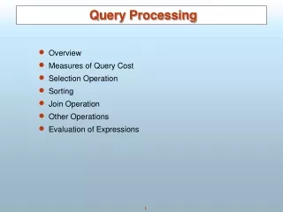
Query Processing Query Execution One-Pass Algorithms Source: our textbook
Overview of Query Processing SQL query parse query query expression tree Query Compilation (Ch 16) select logical query plan Query Optimization logical query plan tree select physical query plan metadata physical query plan tree execute physical query plan Query Execution (Ch 15) data
Overview of Query Compilation • convert SQL query into a parse tree • convert parse tree into a logical query plan • convert logical query plan into a physical query plan: • choose algorithms to implement each operator of the logical plan • choose order of execution of the operators • decide how data will be passed between operations • Choices depend on metadata: • size of the relations • approximate number and frequency of different values for attributes • existence of indexes • data layout on disk
Overview of Query Execution • Operations (steps) of query plan are represented using relational algebra (with bag semantics) • Describe efficient algorithms to implement the relational algebra operations • Major approaches are scanning, hashing, sorting and indexing • Algorithms differ depending on how much main memory is available
Relational Algebra Summary • Set operations: union U, intersection , difference – • projection, PI, (choose columns/atts) • selection, SIGMA, (choose rows/tuples) • Cartesian product X • natural join (bowtie, ) : pair only those tuples that agree in the designated attributes • renaming, RHO, • duplicate elimination, DELTA, • grouping and aggregation, GAMMA, • sorting, TAU,
Measuring Costs • Parameters: • M : number of main-memory buffers available (size of buffer = size of disk block). Only count space needed for input and intermediate results, not output! • For relation R: • B(R) or just B: number of blocks to store R • T(R) or just T: number of tuples in R • V(R,a) : number of distinct values for attribute a appearing in R • Quantity being measured: number of disk I/Os. • Assume inputs are on disk but output is not written to disk.
Scan Primitive • Reads entire contents of relation R • Needed for doing join, union, etc. • To find all tuples of R: • Table scan: if addresses of blocks containing R are known and contiguous, easy to retrieve the tuples • Index scan: if there is an index on any attribute of R, use it to retrieve the tuples
Costs of Scan Operators • Table scan: • if R is clustered, then number of disk I/Os is approx. B(R). • if R is not clustered, number of disk I/Os could be as large as T(R). • Index scan: approx. same as for table scan, since the number of disk I/Os to examine entire index is usually much much smaller than B(R).
Sort-Scan Primitive • Produces tuples of R in sorted order w.r.t. attribute a • Needed for sorting operator as well as helping in other algorithms • Approaches: • If there is an index on a or if R is stored in sorted order of a, then use index or table scan. • If R fits in main memory, retrieve all tuples with table or index scan and then sort • Otherwise can use a secondary storage sorting algorithm (cf. Section 11.4.3)
Costs of Sort-Scan • See earlier slide for costs of table and index scans in case of clustered and unclustered files • Cost of secondary sorting algorithm is: • approx. 3B disk I/Os if R is clustered • approx. T + 2B disk I/Os if R is not
Categorizing Algorithms • By general technique • sorting-based • hash-based • index-based • By the number of times data is read from disk • one-pass • two-pass • multi-pass (more than 2) • By what the operators work on • tuple-at-a-time, unary • full-relation, unary • full-relation, binary
One-Pass, Tuple-at-a-Time • These are for SELECT and PROJECT • Algorithm: • read the blocks of R sequentially into an input buffer • perform the operation • move the selected/projected tuples to an output buffer • Requires only M ≥ 1 • I/O cost is that of a scan (either B or T, depending on if R is clustered or not) • Exception! Selecting tuples that satisfy some condition on an indexed attribute can be done faster!
One-Pass, Unary, Full-Relation • duplicate elimination (DELTA) • Algorithm: • keep a main memory search data structure D (use search tree or hash table) to store one copy of each tuple • read in each block of R one at a time (use scan) • for each tuple check if it appears in D • if not then add it to D and to the output buffer • Requires 1 buffer to hold current block of R; remaining M-1 buffers must be able to hold D • I/O cost is just that of the scan
One Pass, Unary, Full-Relation • grouping (GAMMA) • Algorithm: • keep a main memory search structure D with one entry for each group containing • values of grouping attributes • accumulated values for the aggregations • scan tuples of R, one block at a time • for each tuple, update accumulated values • MIN/MAX: keep track of smallest/largest seen so far • COUNT: increment by 1 • SUM: add value to accumulated sum • AVG: keep sum and count; at the end, divide • write result tuple for each group to output buffer
Costs of Grouping Algorithm • No generic bound on main memory required: • group entries could be larger than tuples • number of groups can be anything up to T but typically • group entries are not longer than tuples • many fewer groups than tuples • Disk I/O cost is that of the scan
One Pass, Binary Operations • Bag union: • copy every tuple of R to the output, then copy every tuple of S to the output • only needs M ≥ 1 • disk I/O cost is B(R) + B(S) • For set union, set intersection, set difference, bag intersection, bag difference, product, and natural join: • read smaller relation into main memory • use main memory search structure D to allow tuples to be inserted and found quickly • needs approx. min(B(R),B(S)) buffers • disk I/O cost is B(R ) + B(S)
Set Union (R U S) • Assume S fits in M-1 main memory buffers • read S into main memory • for each tuple of S • insert it into a search structure D (key is entire tuple) • copy it to output • read each block of R into 1 buffer one at a time • for each tuple of R • if it is not in D (i.e., not in S) then copy to output
Set Intersection (R S) • Assume S fits in M-1 main memory buffers • read S into main memory • for each tuple of S • insert it into a search structure D (key is entire tuple) • read each block of R into 1 buffer one at a time • for each tuple of R • if it is in D (i.e., in S) then copy to output
Set Difference (R - S) • Assume S fits in M-1 main memory buffers • read S into main memory • for each tuple of S • insert into a search structure D (key is entire tuple) • read each block of R into 1 buffer one at a time • for each tuple of R • if it is not in D (i.e., not in S) then copy to output
Additional Binary Operations • See text for one-pass algorithms for • S - R • bag intersection • bag difference • product • Similar to the previous algorithms • Require that one of the operands fit in main memory
One Pass, Natural Join • Assume R(X,Y) is to be joined with S(Y,Z) and S fits in M-1 main memory buffers • read S into main memory • for each tuple of S • insert into a search structure D (key is atts in Y) • read each block of R into 1 buffer one at a time • for each tuple t of R • use D to find all tuples of S that agree with t on atts Y • for each matching tuple u of S, concatenate t and u and copy to output
What Ifs? • What if data is not clustered? • Then it takes T(R) disk I/Os instead of B(R) to read all the tuples of R • But any relation that is the result of an operator will be stored clustered • What if M is unknown/wrongly estimated? • If over-estimated, then one-pass algorithm will be very slow due to thrashing between disk and main memory • If under-estimated and a two-pass algorithm is used when a one-pass would have sufficed, unnecessary disk I/Os are done