Synthetic Curves in Engineering Design
Learn about analytical & synthetic curves, parametric & non-parametric curves, cubic splines, continuity conditions, and piecewise polynomials in engineering design. Discover the importance of curves in engineering design for automobiles, ship hulls, aircraft wings, shoes, propeller blades, bottles, and more.

Synthetic Curves in Engineering Design
E N D
Presentation Transcript
CURVES CAD/CAM/CAE
CURVES Space curve plays important role in engg design: Automobiles ship hulls aircraft wings shoes Propeller blades shoes bottles etc
CURVES • Analytical curve • Curve for which input is standard analytical mathematical equation. • Like point, line, arc, circle, ellipse, parabola etc. • These basic entities can be combined together with various end conditions to generate the overall curve design. • Synthetic curve • It is computed by using geometric input parameters like point, tangent. • These parameters are processed to generate curves. • Bezier , Hermite cubic, B-spline
CURVES • A synthetic curve is described by defining few control points along with additional definitions like tangents etc. • The curve can be generated using point data in two ways: • Interpolation • When resulting curve • necessarily pass through • the point data • Approximation • When the curve does not pass • through the point data but is • controlled smoothly by these points.
NON-PARAMETRIC CURVES • The curve is defined in explicit or implicit form by defining the relationship between the coordinates. • Here a generic point on the curve is defined to generate the curve. • Explicit Form defines the coordinates in terms of other coordinates as follows: x = f ( y, z) y = g ( z, x) z = h ( x, y) • Implicitform are interdependent which cannot be separated: f (x, y, z) = 0 y = 2x-3 2x - y = 3
PARAMETRIC CURVES • Here curve coordinates are defined in terms of single variable called parametric variable. (say u) • If u is parametric variable, then the parametric form of curve is represented by defining the function to define x, y and z independently. x = f ( u) y = g ( u) z = h ( u) • The point (x, y, z) on the curve is defined in terms of independent variable ‘u’. parametric equations of a curve express the coordinates of the points of the curve as functions of a variable, called a parameter x = cos t A common example occurs in kinematics, where the trajectory of a point is usually represented by a parametric equation with time as the parameter.
WHY PARAMETRIC CURVES? • Parametric curves have fewer parameters for smooth surfaces. • Fewer parameters makes it faster to create a curve, and easier to edit an existing curve. • Parametric curves are easier to animate. • Parametric representation can be used for both A & S curves. • All coordinates are defined independently.
Types of Synthetic Curves 1. Cubic spline 2. Bezier Curve 3. B-spline Curve
CUBIC SPLINE A spline curve is a mathematical representation for which it is easy to build an interface that will allow a user to design and control the shape of complex curves and surfaces. Splines are smooth curves passing through a given set of points. The general approach is that the user enters a sequence of points, and a curve is constructed whose shape closely follows this sequence. The points are called control points.
CUBIC SPLINE Offer compromise between flexibility and speed of computation Compared to higher order polynomial: CS require less calculation less memory are more stable Compared to lower order polynomial: CS are more flexible for modeling arbitrary curve shapes
CONTINUITY CONDITION • A synthetic curve can be generated by combining numbers of small synthetic curve segments. • i.e. the curve S may be generated by joining S1, S2 ….Sn • These segments are joined together end to end to generate a complex synthetic curve. • The order of the continuity determines the smoothness of joining and hence the total curve. • If there are two consecutive segments , the condition of the end segments can be defined in three different ways.
CONTINUITY CONDITION Condition: C0 continuity • Each curve start with the previous one ends. • the two segments match values at the join. Condition: C1 continuity • The slopes have to match at the common endpoints. • So set first derivatives equal. Condition: C2 continuity • Provides better smoothing. • Gives us a unique solution. • they match curvatures at the join.
Piecewise Polynomial • When the polynomials are joined at adjacent intervals to form a continuous curve, it is named as piecewise polynomial. • The figure shows a curve q(u) that consists of four polynomials: l(u), m(u), n(u) k(u) • l(u) = 1/6 u3 • m(u) = 1/6 u2 (2-u) + 1/6 u (u-1)(3-u) + 1/6 (u-1)2 (4-u) • n(u) = 1/6 u (3-u) 2 + 1/6 (4-u)(u-1)(3-u) + 1/6 (u-2) (4-u) 2 • k(u) = 1/6 (4-u)3
Piecewise Polynomial • The support q(u) is [0,4] • where l(u) is defined on the span [0,1] • m(u) is defined on the span [1,2] • n(u) is defined on the span [2,3] • k(u) is defined on the span [3,4] • The points where individual segments meets is known as joints. • The values of u at which a pair of the individual segments meet are called as knots.
Piecewise Polynomial • To find whether q(u) is continuous everywhere over its support? • It is continuous inside each span as it is built from polynomials. • Need to check if adjacent segments meet properly at joints. • For u = 1 ; l(1) = m (1) = 1/6 • For u = 2 ; m(2) = n (2) = 2/3 • For u = 3 ; n(3) = k (3) = 1/6 • To check first derivatives of q(u) (only at knots) • For u = 1 ; l'(1) = m' (1) • For u = 2 ; m'(2) = n' (2) • For u = 3 ; n'(3) = k '(3) • To check second derivatives of q(u) • For u = 1 ; l''(1) = m'' (1) • For u = 2 ; m''(2) = n'' (2) • For u = 3 ; n''(3) = k ''(3) • Piecewise polynomial of three degree. (cubic spline) Showing C0 continuity Showing C1 continuity Showing C2 continuity
Hermite Cubic Curve • It is named after the French mathematician Charles Hermite. • It is a synthetic curve with cubic degree which generates an interpolated curve. • This sort of curve is used to generate simple curves and is not used to generate free form curves with enhanced controllability. • The curve is synthesized using two extreme data points (start and end) and tangents at these end points. • As Hermite cubic curve is having cubic degree it may be written as
Key features of Hermite Cubic Curve • It is a parametric cubic curve. • It can generate a long curve by combining the number of curves but it can provide only C0 continuity. • It is an interpolation type of curve and hence it is not used to generate free form shapes. • Two points and two slopes at the start and end points are used as input. • Defining tangents is not very convenient.
Inference from Hermite Cubic Curve equation • It is a cubic spline curve in terms of its two end points and their tangent vectors. • The equation shows that the curve passes through the end points u = 0 and u = 1. • It also shows that the curve shape can be controlled by changing its end points or tangent vectors. • If two end points are fixed in space then the designer can control the shape of the spline by either changing the magnitude or direction of tangent vectors.
Inference from Hermite Cubic Curve equation • Equation of P(u) is for one cubic spline segment. • It can be generalized for any two adjacent spline segments of a spline curve that are to fit a given number of data points. • This introduces the problem of joining cubic spline segments.
INTRODUCTION • In Engineering, one often wants a smooth curve through a set of known points. • In Physics, a smooth curve is required to represent the shape of a deflected beam. • Computer Aided Design and Manufacturing programs--- like lines and circular arcs. • Bezier Curves were first developed in 1959 by Paul de Casteljau. • They were popularized in 1962 by French engineer Pierre Bezier, who used them to design automobile bodies. • M. Bezier was a French mathematician who worked for the Renault motor car company. • He invented this curves to allow his firm’s computers to describe the shape of car bodies.
An alternative to splines. • The shape of Bezier curve is controlled by its defining points only. This allows the designer a much better feel for the relationship between input (points) and output (arcs). • The order or the degree of the curve is variable and is related to the number of points defining it: • n + 1 points define an nth degree curve. • Need four points • Two at the ends of a segment • Two control tangent vectors • The Bezier curve is smoother than other curve as it has higher order derivative.
The Bezier curve is defined in terms of location of n+1 point. • These points are called as data or control points. • They form the vertices of what is called the control or Bezier characteristics polygon which uniquely defines the curve shape as shown in figure. • Only the first and last vertices point lie on the curve. • The other vertices define the order, derivatives and shapes of the curve. • The curve is also tangent to the first and last polygon segments. • Also the curve shape tends to follow the polygon shape.
The figure shows the order of defining the control points changes the polygon definition which changes the resulting curve shape.
BEZIER CURVE PROPERTIES • The first and last control points are interpolated. • Put u = 0 and 1 in equation , we will get Po and P1 • The curve is tangent to the first and last segment of the characteristic polygon. • The tangent at the last control point is along the line joining the second last and last control points • Not all of the control points are on the line • Some just attract it towards themselves • The curve lies entirely within the convex hull of its control points
BEZIER CURVE PROPERTIES • The curve can be modified by either changing one or more vertices of its polygon or by keeping the polygon fixed and specifying multiple coincident points at a vertex. • sketch • A closed Bezier curve can be generated by simply closing its characteristic polygon or choosing Po and Pn to be coincident.
Convex hull • Convex polygon formed by connecting the control points of the curve. • The curve lies entirely within the convex hull of its control points. • If the control vertices are nearly collinear, then the convex hull is a good approximation to the curve
CHARACTERISTICS OF BEZIER CURVES: • Curves that posses convex hull property have foll. consequences. 1. If the polygon defining a curve segment degenerates to a straight line, the curve must then be a straight line. • Thus BC may have locally linear segment embedded in it. 2. The size of convex hull is the upper bound to the curve. • this property can be used for clipping, where instead of testing the curve, the polygon can first be tested 3.The curve never oscillates wildly away from its defining control points as it is guaranteed to lie within its convex hull.
What does it mean ? 1 0 1
p(t) = (1-t)3p0 + 3(1-t)2tp1 + 3(1-t)t2p2 + t3p3 = (1 – 3t + 3t2 – t3) p0 + (3t – 6t2 + 3t3)p1 + (3t2 –3t3)p2 + t3 p3
Disadvantages • The degree of the Bezier curve depends on the number of control points. • The Bezier curve lacks local control. • Changing the position of one control point affects the entire curve. (designer cannot selectively change part of curve.) • Expensive to evaluate the curve at many points • No easy way of knowing how fine to sample points, and may be sampling rate must be different along curve. • No easy way to adapt. In particular, it is hard to measure the deviation of a line segment from the exact curve.
CHARACTERISTICS OF B-SPLINE CURVES: 1. The local control of the curve can be achieved by • changing the position of the control point(s) • Using multiple control points by placing several points at the same location • By choosing different degree (k-1)
CHARACTERISTICS OF B-SPLINE CURVES: 2. A non-periodic B-spline curve passes through the first and last control points P0 and Pn+1 and is tangent to the first (P1-P0) and last (Pn+1 – Pn) segments of the control polygon.
CHARACTERISTICS OF B-SPLINE CURVES: • 3. Increasing the degree of curve tightens it. • The lesser the degree, the closer the curve gets to the control points. • For k=1, a zero degree curve results (curve itself becomes the control point) • For k=2, curve become the polygon segments themselves.
CHARACTERISTICS OF B-SPLINE CURVES: • 4. A second degree curve is always tangent to the midpoints of • all the internal polygon segments. • This is not the case for other curves.
CHARACTERISTICS OF B-SPLINE CURVES: 5. If k= no of CPs (n+1), then the resulting B-spline curve becomes Bezier curve. in this case the range of u becomes zero to one.
CHARACTERISTICS OF B-SPLINE CURVES: 6. Multiple control points induce regions of high curvature of B-spline curve. This is useful when creating sharp corners in the curve. the effect is equivalent to saying that the curve is pulled more towards a control points by increasing its multiplicity.
CHARACTERISTICS OF B-SPLINE CURVES: 7. Increasing the degree of curve makes it more difficult to control and to calculate accurately. • Therefore a cubic B-spline curve is sufficient for a large number of applications.