Download
1 / 23
230 likes | 260 Vues
This introduction to diffusion MRI explains how water molecule motion can differentiate brain tissues. It covers encoding methods, tensor modeling, and interpreting diffusion measurements. Learn about isotropic and anisotropic diffusion, tensor imaging, and measures derived from eigenvalues. Discover how gradient directions and b-values impact data quality and image acquisition. Master the applications and significance of diffusion MRI in neurology, including tracking neurodegenerative diseases, stroke, and aging. This valuable tool aids in understanding brain structure at the microscopic level, offering insight into various biological processes.

E N D
Introduction to diffusion MRI Anastasia Yendiki HMS/MGH/MIT Athinoula A. Martinos Center for Biomedical Imaging
White-matter imaging • Axons measure ~m in width • They group together in bundles that traverse the white matter • We cannot image individual axons but we can image bundles with diffusion MRI • Useful in studying neurodegenerative diseases, stroke, aging, development… From the National Institute on Aging From Gray's Anatomy: IX. Neurology
Diffusion in brain tissue • Differentiate tissues based on the diffusion (random motion) of water molecules within them • Gray matter: Diffusion is uniformly restricted isotropic • White matter: Diffusion is preferentially restricted anisotropic
Diffusion MRI Diffusion encoding in direction g1 • Magnetic resonance imaging can provide “diffusion encoding” • Magnetic field strength is varied by gradients in different directions • Image intensity is attenuated depending on water diffusion in each direction • Compare with baseline images to infer on diffusion process g2 g3 g4 g5 g6 No diffusion encoding
How to represent diffusion • At every voxel we want to know: • Is this in white matter? • If yes, what pathway(s) is it part of? • What is the orientation of diffusion? • What is the magnitude of diffusion? • A grayscale image cannot capture all this!
d11 d12 d13 d12d22 d23 d13 d23d33 D = Tensors • One way to express the notion of direction is a tensor D • A tensor is a 3x3 symmetric, positive-definite matrix: • D is symmetric 3x3 It has 6 unique elements • Suffices to estimate the upper (lower) triangular part
eix eiy eiz ei = Eigenvalues & eigenvectors • The matrixD is positive-definite • It has 3 real, positive eigenvalues 1, 2, 3> 0. • It has 3 orthogonal eigenvectors e1, e2, e3. 1e1 2e2 3e3 D= 1e1 e1´ + 2e2 e2´ + 3e3 e3´ eigenvalue eigenvector
Physical interpretation • Eigenvectors express diffusion direction • Eigenvalues express diffusion magnitude Isotropic diffusion: 123 • Anisotropic diffusion: • 1>>2 3 1e1 1e1 2e2 3e3 2e2 3e3 • One such ellipsoid at each voxel: Likelihood of water molecule displacements at that voxel
Diffusion tensor imaging (DTI) Image: An intensity valueat each voxel Tensor map: A tensorat each voxel Direction of eigenvector corresponding to greatest eigenvalue
Diffusion tensor imaging (DTI) Image: An intensity valueat each voxel Tensor map: A tensorat each voxel Direction of eigenvector corresponding to greatest eigenvalue Red: L-R, Green: A-P, Blue: I-S
Tensor-based measures Faster diffusion • Mean diffusivity (MD): • Mean of the 3 eigenvalues Slower diffusion MD(j) = [1(j)+2(j)+3(j)]/3 Anisotropic diffusion • Fractional anisotropy (FA):Variance of the 3 eigenvalues, normalized so that0 (FA) 1 Isotropic diffusion [1(j)-MD(j)]2+ [2(j)-MD(j)]2+ [3(j)-MD(j)]2 3 FA(j)2 = 1(j)2+ 2(j)2+ 3(j)2 2
Tensor-based measures • Axial diffusivity: Greatest of the 3 eigenvalues • Radial diffusivity: Average of 2 lesser eigenvalues AD(j) = 1(j) RD(j) = [2(j) + 3(j)]/2 • Different biological processes can have the same effect on these measures: • Myelination anisotropy • Axon coherence anisotropy
Choice 1: Gradient directions • True diffusion direction || Applied gradient direction Maximum attenuation • True diffusion direction Applied gradient direction No attenuation • To capture all diffusion directions well, gradient directions should cover 3D space uniformly Diffusion-encoding gradient g Displacement detected Diffusion-encoding gradient g Displacement not detected Diffusion-encoding gradient g Displacement partly detected
How many directions? • Acquiring data with more gradient directions leads to: • More reliable estimation of diffusion measures • Increased imaging time Subject discomfort, more susceptible to artifacts due to motion, respiration, etc. • DTI: • Six directions is the minimum • Usually a few 10’s of directions • Diminishing returns after a certain number [Jones, 2004] • DSI: • Usually a few 100’s of directions
Choice 2: The b-value • The b-value depends on acquisition parameters: b = 2G22 (- /3) • the gyromagnetic ratio • G the strength of the diffusion-encoding gradient • the duration of each diffusion-encoding pulse • the interval b/w diffusion-encoding pulses 90 180 acquisition G
How high b-value? • Increasing the b-value leads to: • Increased contrast b/w areas of higher and lower diffusivity in principle • Decreased signal-to-noise ratio Less reliable estimation of diffusion measures in practice • DTI: b ~ 1000 sec/mm2 • DSI: b ~ 10,000 sec/mm2 • Data can be acquired at multiple b-values for trade-off • Repeat acquisition and average to increase signal-to-noise ratio
Looking at the data A diffusion data set consists of: • A set of non-diffusion-weighted a.k.a “baseline” a.k.a. “low-b” images (b-value = 0) • A set of diffusion-weighted (DW) images acquired with different gradient directions g1, g2, … and b-value >0 • The diffusion-weighted images have lower intensity values b2, g2 b3, g3 b=0 b1, g1 Baseline image Diffusion-weighted images b4, g4 b5, g5 b6, g6
Distortions: Field inhomogeneities Signal loss • Causes: • Scanner-dependent (imperfections of main magnetic field) • Subject-dependent (changes in magnetic susceptibility in tissue/air interfaces) • Results: • Signal loss in interface areas • Geometric distortions (warping) of the entire image
Distortions: Eddy currents • Cause: Fast switching of diffusion-encoding gradients induces eddy currents in conducting components • Eddy currents lead to residual gradients that shift the diffusion gradients • The shifts are direction-dependent,i.e., different for each DW image • Result: Geometric distortions From Le Bihan et al., Artifacts and pitfalls in diffusion MRI, JMRI 2006
Data analysis steps • Pre-process images to reduce distortions • Either register distorted DW images to an undistorted (non-DW) image • Or use information on distortions from separate scans (field map, residual gradients) • Fit a diffusion model at every voxel • Tensor, ball-and-stick, ODF, … • Do tractography to reconstruct pathways and/or • Compute measures of anisotropy/diffusivity and compare them between populations • Voxel-based, ROI-based, or tract-based statistical analysis
Caution! • The FA map or color map is not enough to check if your gradient table is correct - display the tensor eigenvectors as lines • Corpus callosum on a coronal slice, cingulum on a sagittal slice
Tutorial • Use dt_recon to prepare DWI data for a simple voxel-based analysis: • Calculate and display FA/MD/… maps • Intra-subject registration (individual DWI to individual T1) • Inter-subject registration (individual T1 to common template) • Use anatomical segmentation (aparc+aseg) as a brain mask for DWIs • Map all FA/MD/… volumes to common template to perform voxel-based group comparison