Download
1 / 50
560 likes | 866 Vues
Applied Hydrology Climate Change and Hydrology (I) - GCMs and Climate Change Scenarios. Professor Ke-Sheng Cheng Department of Bioenvironmental Systems Engineering National Taiwan University. Climate dynamics, climate change and climate prediction.

E N D
Applied HydrologyClimate Change and Hydrology(I) - GCMs and Climate Change Scenarios Professor Ke-Sheng Cheng Department of Bioenvironmental Systems Engineering National Taiwan University
Climate dynamics, climate change and climate prediction • Climate: average condition of the atmosphere, ocean, land surfaces and the ecosystems in them. • e.g., "Baja California has a desert climate” • Weather: state of atmosphere and ocean at given moment. • Climate includes average measures of weather-related variability. • e.g., probability of a major rainfall event occurring in July in Baja, variations of temperature that typically occur during January in Chicago, … Neelin, 2011. Climate Change and Climate Modeling Lab for Remote Sensing Hydrology and Spatial Modeling Dept of Bioenvironmental Systems Eng, NTU
Climate quantities defined by averaging over the weather • Average taken over January of many different years to obtain a climatological value for January, many Februaries to obtain February climatology, etc. Climatology of sea surface temperature for January (15 year average) Neelin, 2011. Climate Change and Climate Modeling, Cambridge UP
Climate change: • occurring on many time scales, including those that affect human activities. • time period used in the average will affect the climate that one defines. • e.g., 1950-1970 will differ from the average from 1980-2000. • Climate variability: • essentially all the variability that is not just weather. • e.g., ice ages, warm climate at the time of dinosaurs, drought in African Sahel region, and El Niño. Climate change usually refers to changes in statistical properties of climate variables. A stationary climate process can and usually do exhibit climate variability. Neelin, 2011. Climate Change and Climate Modeling, Cambridge UP
Anthropogenic climate change: due to human activities. • e.g., ozone hole, acid rain, and global warming. Data from the Program for Model Diagnosis and Intercomparison (PCMDI) archive. Neelin, 2011. Climate Change and Climate Modeling, Cambridge UP
Global warming: predicted warming, & associated changes in the climate system in response to increases in "greenhouse gases" emitted into atmosphere by human activities. • Greenhouse gases: e.g., carbon dioxide, methane and chlorofluorocarbons: trace gases that absorb infrared radiation, affect the Earth's energy budget. • warming tendency, known as the greenhouse effect • Global change: human-induced changes more generally (including ozone hole). • Environmental change: even more general (including air, water pollution, deforestation, ecosystems change, …) • Climate prediction endeavor to predict not only human-induced changes but the natural variations. e.g., El Niño Neelin, 2011. Climate Change and Climate Modeling, Cambridge UP
Climate Dynamics or Climate Science: studies climate and climate change processes (older term, “climatology”). • Climatology now used for average variables, e.g., “the January precipitation climatology”. • Climate models: • Mathematical representations of the climate system • typically equations for temperature, winds, ocean currents and other climate variables solved numerically on computers. • Climate System or Earth System: global, interlocking system; atmosphere, ocean, land surfaces, sea and land ice, and biosphere (plant and animal component). Neelin, 2011. Climate Change and Climate Modeling, Cambridge UP
Changes in climate/weather • Climate extremes or weather extremes? • Extreme rainfalls are results of severe weather events. • Changes in climate can affect occurrences and frequencies of extreme weather events. • Studies which evaluate the impact of climate change on rainfall extremes by comparing to rainfall climatology may be misleading. 2013 AsiaFlux, HESSS, GCEER, KSAFM Joint Conference
Climate extremes and weather extremes 2013 AsiaFlux, HESSS, GCEER, KSAFM Joint Conference
Climate extremes 2013 AsiaFlux, HESSS, GCEER, KSAFM Joint Conference
Weather extremes 2013 AsiaFlux, HESSS, GCEER, KSAFM Joint Conference
Climate models - a brief overview • Motions, temperature, etc. governed by basic laws of physics solved numerically: • e.g., divide the atmosphere and ocean into discrete grid boxes • equation for balance of forces, energy inputs etc. for each box. • obtain the acceleration of the fluid in the box, its rate of change of temperature, etc. • from this compute the new velocity, temperature, etc. one time step later (e.g., twenty minutes for the atmosphere, hour for ocean). • equations for each box depend on the values in neighboring boxes. • computation is done for a million or so grid boxes over the globe. • repeated for the next time step, and so on until the desired length of simulation is obtained. • common to simulate decades or centuries in climate runs • computational cost a factor Neelin, 2011. Climate Change and Climate Modeling, Cambridge UP
Also close relationship to weather forecasting models • Major differences: • complexity of the climate system. • range of phenomena at different time scales. • “messier”: clouds, aerosols, vegetation, ... • More attention to processes that affect the long term Neelin, 2011. Climate Change and Climate Modeling, Cambridge UP
The most complex climate models, known as General Circulation Models or GCMs. • Once a phenomena has been simulated in a GCM, it is not necessarily easy to understand. • Intermediate complexity climate models are also used. • construct a model based on same physical principles as a GCM but only aspects important to the target phenomenon are retained. • e.g., first used to simulate, understand and predict El Niño. • Simple climate models: • e.g., globally averaged energy-balance model, to understand essential aspects of the greenhouse effect. • Global warming simulations with GCMs Þ detailed processes, 3-D response. Neelin, 2011. Climate Change and Climate Modeling, Cambridge UP
Global mean surface temperatures estimated since preindustrial times From the University of East Anglia CRU (data following Brohan et al. 2006; Rayner et al. 2006) • Anomalies relative to 1961-1990 mean • Annual average values of combined near-surface air temperature over continents and sea surface temperature over ocean. • Curve: smoothing similar to a decadal running average. Neelin, 2011. Climate Change and Climate Modeling, Cambridge UP
Anomaly:departure from normal climatological conditions. • calculated by difference between value of a variable at a given time, e.g., pressure or temperature for a particular month, and subtracting the climatology of that variable. • Climatology includes the normal seasonal cycle. • e.g., anomaly of summer rainfall for June, July and August 1997, = average of rainfall over that period minus averages of all June, July and August values over a much longer period, such as 1950-1998. • To be precise, the averaging time period for the anomaly and the averaging time period for the climatology should be specified. • e.g., monthly averaged SST anomalies relative to 1950-2000 mean. Neelin, 2011. Climate Change and Climate Modeling, Cambridge UP
Global Circulation Models (GCMs) • Computer models that • are capable of producing a realistic representation of the climate, and • can respond to the most obvious quantifiable perturbations. • Derived based on weather forecasting models. Lab for Remote Sensing Hydrology and Spatial Modeling Dept of Bioenvironmental Systems Eng, NTU
Weather forecasting models • The physical state of the atmosphere is updated continually drawing on observations from around the world using surface land stations, ships, buoys, and in the upper atmosphere using instruments on aircraft, balloons and satellites. • The model atmosphere is divided into 70 layers and each level is divided up into a network of points about 40 km apart. Lab for Remote Sensing Hydrology and Spatial Modeling Dept of Bioenvironmental Systems Eng, NTU
Standard weather forecasts do not predict sudden switches between stable circulation patterns well. At best they get some warning by using statistical methods to check whether or not the atmosphere is in an unpredictable mood. This is done by running the models with slightly different starting conditions and seeing whether the forecasts stick together or diverge rapidly. Lab for Remote Sensing Hydrology and Spatial Modeling Dept of Bioenvironmental Systems Eng, NTU
This ensemble approach provides a useful indication of what modelers are up against when they seek to analyses the response of the global climate to various perturbations and to predict the course it will following in the future. • The GCMs cannot represent the global climate in the same details as the numerical weather predictions because they must be run for decades and even centuries ahead in order to consider possible changes. Lab for Remote Sensing Hydrology and Spatial Modeling Dept of Bioenvironmental Systems Eng, NTU
Typically, most GCMs now have a horizontal resolution of between 125 and 400 km, but retain much of the detailed vertical resolution, having around 20 levels in the atmosphere. • Challenges for potential GCMs improvement • Modeling clouds formation and distribution • Tropical storms (typhoons and hurricanes) • Land-surface processes • Winds, waves and currents • Other greenhouse gases Lab for Remote Sensing Hydrology and Spatial Modeling Dept of Bioenvironmental Systems Eng, NTU
GCMs Lab for Remote Sensing Hydrology and Spatial Modeling Dept of Bioenvironmental Systems Eng, NTU
The parameterization problem • For each grid box in a climate model, only the average across the grid box of wind, temperature, etc. is represented. • In the observations, many fine variations occur inside, • e.g., squall lines, cumulonimbus clouds, etc. • The average of these small scale effects has important impacts on large-scale climate. • e.g., clouds primarily occur at small scales, yet the average amount of sunlight reflected by clouds affects the average solar heating of a whole grid box. • Average effects of the small scales on the grid scale must be included in the climate model. • These averages change with the parameters of large-scale fields that affect the clouds, such as moisture and temp. Neelin, 2011. Climate Change and Climate Modeling, Cambridge UP
Method of representing average effects of clouds (or other small scale effects) over a grid box interactively with the other variables known as parameterization. • Successes and difficulties of parameterization important to accuracy of climate models. • finer grid implies greater computational costs (or shorter simulation) • As computers become faster Þ finer grids. • But there are always smaller scales. • Scale interaction is one of the main effects that makes climate modeling challenging. Neelin, 2011. Climate Change and Climate Modeling, Cambridge UP
Constructing a Climate Model Typical atmospheric GCM grid • For each grid cell, single value of each variable (temp., vel.,…) ÞFinite number of equations • Vertical coordinate follows topography, grid spacing varies • Transports (fluxes) of mass, energy, moisture into grid cell ÞBudget involving immediate neighbors (in balance of forces, PGF involves neighbors) • Effects passed from neighbor to neighbor until global • Budget gives change of temperature, velocity, etc., one time step (e.g. 15 min) later • 100yr=4million 15min steps Figure 5.1 Neelin, 2011. Climate Change and Climate Modeling, Cambridge UP
Treatment of sub-grid scale processes Vertical column showing parameterized physics so smallscale processes within a single column in a GCM Neelin, 2011. Climate Change and Climate Modeling, Cambridge UP
Resolution and computational cost Topography of western North America at 0.3° and 3.0° resolutions Neelin, 2011. Climate Change and Climate Modeling, Cambridge UP
Topography of North America at 0.5° and 5.0° resolutions Neelin, 2011. Climate Change and Climate Modeling, Cambridge UP
Resolution and computational cost • Computational time = (computer time per operation) ´(operations per equation)´(No. equations per grid-box) ´(number of grid boxes)´(number of time steps per simulation) • Increasing resolution: # grid boxes increases & time step decreases • Half horizontal grid size Þ half time step Þ twice as many time steps to simulate same number of years • Doubling resolution in x, y & z Þ 2´2´2´(# grid cells) ´2´(# of time steps) Þ cost increases by factor of 24 =16 • Increase horizontal resolution, 5 to 0.5 degrees Þ factor of 10 in each horizontal direction. So even if kept vertical grid same,10´10´(# grid cells)´10´(# of t steps)= 103 • Suppose also double vertical res. Þ 2000 times the computational time i.e. costs same to run low-res. model for 40 years as high res. for 1 week • To model clouds, say 50m res. Þ 10000 times res. in horizontal, if same in vertical and time Þ 1016 times the computational time … and will still have to parameterize raindrop, ice crystal coalescence etc. Neelin, 2011. Climate Change and Climate Modeling, Cambridge UP
Why time step must decrease when grid size decreases: • Time step must be small enough to accurately capture time evolution and for smaller grid size, smaller time scales enter. • A key time scale: time it takes wind or wave speed to cross a grid box. e.g., if fastest wind 50 m/s, crosses 200 km grid box in ~ 1 hour • If time step longer, more than 1 grid box will be crossed: can yield amplifying small scale noise until model “blows up” (for accuracy, time step should be significantly shorter) Neelin, 2011. Climate Change and Climate Modeling, Cambridge UP
Finite differencing of a pressure field Numerical representation of atmos. and oceanic eqns. Finite difference versus spectral models Neelin, 2011. Climate Change and Climate Modeling, Cambridge UP
Spectral representation of a pressure field Neelin, 2011. Climate Change and Climate Modeling, Cambridge UP
Climate drift Climate simulations and climate drift Examples of model integrations (or runs, simulations or experiments), starting from idealized or observed initial conditions. Spin-up to equilibrated model climatology is required (centuries for deep ocean). Model climate differs slightly from observed (model error aka climate drift); climate change experiments relative to model climatology. Neelin, 2011. Climate Change and Climate Modeling, Cambridge UP
Commonly used scenarios Radiative forcing as a function of time for various climate forcing scenarios Top of the atmosphere radiative imbalance Þwarming due to the net effects of GHG and other forcings from the Special Report on Emissions Scenarios • SRES: • A1FI (fossil intensive), • A1T (green technology), • A1B (balance of these), • A2,B2(regional economics) • B1 “greenest” • IS92a scenario used in many • studies before 2005 Adapted from Meehl et al., 2007 in in IPCC Fourth Assessment Report Neelin, 2011. Climate Change and Climate Modeling, Cambridge UP
SRES emissions scenarios, cont’d A1 scenario family: assumes low population growth, rapid economic growth, reduction in regional income differences A1FI : Fossil fuel Intensive A1B: energy mix, incl. non-fossil fuel A2: uneven regional economic growth, high income toward non-fossil, population 15 billion in 2100 B1: like A1 but switch to information and service economy, introduction of resource-efficient technology. Emphasis on global solutions to economic, social, and environmental sustainability, including improved equity. • No explicit consideration of treaties • Natural forcings e.g., volcanoes set to avg. from 20th C. Neelin, 2011. Climate Change and Climate Modeling, Cambridge UP
CCMA_CGCM3.1, Canadian Community Climate Model • CNRM_CM3, Meteo-France, Centre National de Recherches Meteorologiques • CSIRO_MK3.0, CSIRO Atmospheric Research, Australia • GFDL_CM2.0, NOAA Geophysical Fluid Dynamics Laboratory • GFDL_CM2.1, NOAA Geophysical Fluid Dynamics Laboratory • GISS_ER, NASA Goddard Institute for Space Studies, ModelE20/Russell • MIROC3.2_medres, CCSR/NIES/FRCGC, medium resolution • MPI_ECHAM5, Max Planck Institute for Meteorology, Germany • MRI_CGCM2.3.2a, Meteorological Research Institute, Japan • NCAR_CCSM3.0, NCAR Community Climate System Model • NCAR_PCM1, NCAR Parallel Climate Model (Version 1) • UKMO_HADCM3, Hadley Centre for Climate Prediction, Met Office, UK Model names (a sample) Neelin, 2011. Climate Change and Climate Modeling, Cambridge UP
Global average warming simulations in 11 climate models • Global avg. sfc. air temp. change • (ann. means rel. to 1901-1960 base period) • Est. observed greenhouse gas + aerosol forcing, followed by • SRES A2 scenario (inset) in 21st century • (includes both GHG and aerosol forcing) Data from the Program for Model Diagnosis and Intercomparison (PCMDI) archive. Neelin, 2011. Climate Change and Climate Modeling, Cambridge UP
Spatial patterns of the response to time-dependent warming scenarios Response to the SRES A2 scenario GHG and sulfate aerosol forcing in surface air temperature relative to the average during 1961-90 from the Hadley Centre climate model (HadCM3)[choosing one model simulation through the 21st century as an example; later compare models or average results from several models] 2010-2039 2040-2069 2070-2099 Figure 7.5 Neelin, 2011. Climate Change and Climate Modeling, Cambridge UP
Response to the SRES A2 scenario GHG and sulfate aerosol forcing in surface air temperature relative to the average during 1961-90 from the National Center for Atmospheric Research Community Climate Simulation Model (NCAR_CCSM3) 2010-2039 2040-2069 2070-2099 Neelin, 2011. Climate Change and Climate Modeling, Cambridge UP
January January and July surface temperature from HadCM3 averaged 2040-2069 (SRES A2 scenario) July Neelin, 2011. Climate Change and Climate Modeling, Cambridge UP
January January and July surface temperature from NCAR_CCSM3 averaged 2040-2069 (SRES A2 scenario) July Neelin, 2011. Climate Change and Climate Modeling, Cambridge UP
Comparing projections of different climate models 30yr. avg annual surface air temperature response for 3 climate models centered on 2055 relative to the average during 1961-1990 GFDL- CM2.0 NCAR- CCSM3 MPI- ECHAM5 Figure 7.7 Neelin, 2011. Climate Change and Climate Modeling, Cambridge UP
Comparing projections of different climate models • Provides estimate of uncertainty • Differences often occur with physical processes e.g., shift of jet stream, reduction of soil moisture, … • At regional scales (~size of country or state) more disagreement • Precip challenging at regional scales Neelin, 2011. Climate Change and Climate Modeling, Cambridge UP
Comparing projections of different climate models GFDL- CM2.0 Precipitation from 3 models for Jun.-Aug. 2070-2099 average minus 1961-90 avg (SRES A2 scenario) NCAR- CCSM3 MPI- ECHAM5 (mm/day) Neelin, 2011. Climate Change and Climate Modeling, Cambridge UP
Comparing projections of different climate models Precipitation from 3 models for Dec.-Feb. 2070-2099 average minus 1961-90 avg (SRES A2 scenario) GFDL- CM2.0 NCAR- CCSM3 MPI- ECHAM5 (mm/day) Neelin, 2011. Climate Change and Climate Modeling, Cambridge UP
Precipitation from HadCM3 for Dec.-Feb. 2070-2099 avg. (SRES A2) Neelin, 2011. Climate Change and Climate Modeling, Cambridge UP
Precipitation from HadCM3 for Jun.-Aug. 2070-2099 avg. (SRES A2) Neelin, 2011. Climate Change and Climate Modeling, Cambridge UP
From GCMs to hydrological process modeling • Study of hydrological processes requires spatial and temporal resolutions which are much smaller than GCMs can offer. • Downscaling techniques have been developed to downscale GCM outputs to desired scales. • Dynamic downscaling • Statistical downscaling Lab for Remote Sensing Hydrology and Spatial Modeling Dept of Bioenvironmental Systems Eng, NTU
Lab for Remote Sensing Hydrology and Spatial Modeling Dept of Bioenvironmental Systems Eng, NTU