Instrumental Analysis
This resource offers a detailed overview of instrumental analysis, covering key techniques such as atomic absorption, fluorescence spectroscopy, UV/Vis spectroscopy, and more. Expert instructors including Upali Siriwardane and Frank Ji guide students through intricate concepts, emphasizing the importance of experimental design, precision, and accuracy. The course utilizes the required text "Principles of Instrumental Analysis" (5th Edition) by Skoog, Holler, and Nieman, ensuring a thorough understanding of analytical methods, error analysis, and chromatography applications.

Instrumental Analysis
E N D
Presentation Transcript
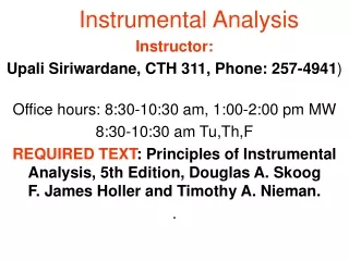
Instrumental Analysis Instructors: Upali Siriwardane, CTH 311, Phone: 257-4941) Frank Ji, CTH 343/IfM 218, Phone: 257-4066/5125 Dale L. Snow, Office:CTH 331,Phone: 257-4403 Jim Palmer, BH 5 /IfM 121, Phone: 572885/5126 Bill Elmore, BH 222 /IfM 115 Phone: 257-2902/5143 Marilyn B. Cox, Office: CTH 337, Phone: 257-4631 REQUIRED TEXT: Principles of Instrumental Analysis, 5th Edition, Douglas A. Skoog F. James Holler and Timothy A. Nieman. .
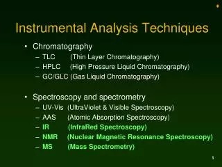
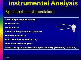
Content Atomic Absorption & Fluorescence Spectroscopy (Upali) 6. An Introduction to Spectrometric Methods. 9. Atomic Absorption and Atomic Fluorescence Spectrometry. Ultraviolet/Visible Spectroscopy(Snow) 13. An Introduction to Ultraviolet/Visible Molecular Absorption Spectrometry. 14. Applications of Ultraviolet/Visible Molecular Absorption Spectrometry. Infrared Spectrometry( Frank Ji) 16. An Introduction to Infrared Spectrometry. 17. Applications of Infrared Spectrometry. Nuclear Magnetic Resonance Spectroscopy) (Upali)19. Nuclear Magnetic Resonance Spectroscopy. Mass Spectrometry (Palmer/Upali/Cox20. Molecular Mass Spectrometry. Gas Chromatography ( JimPalmer) 26. An Introduction to Chromatographic Separations. 27. Gas Chromatography. High-Performance Liquid Chromatography (Bill Elmore)28. High-Performance Liquid Chromatography. Special Topics (Upali) 12. Atomic X-Ray Spectrometry. 31. Thermal Methods
Analytical Chemistry • art of recognizing different substances & determining their constituents, takes a prominent position among the applications of science, since the questions it enables us to answer arise wherever chemical processes are present. • 1894 Wilhelm Ostwald
You don’t need a course to tell you how to run an instrument • They are all different and change • Most of you won’t be analysts • We will talk about experimental design • Learn about the choices available and the basics of techniques
Questions to ask??? • Why? Is sample representative • What is host matrix? • Impurities to be measured and approximate concentrations • Range of quantities expected • Precision & accuracy required
Off flavor cake mix (10%) • Send it off for analysis • Do simple extractions • Separation and identification by GC/MS • Over 100 peaks but problem was in a valley between peaks (compare) • Iodocresol at ppt • Eliminate iodized salt that reacted with food coloring (creosol=methyl phenol)
• The digits in a measured quantity that are known exactly plus one uncertain digit. 29.42 mL Certain + one uncertain 29.4 mL Certain I. Significant Figures
Rule 1: To determine the number of significant figures in a measurement, read the number from left to right and count all digits, starting with the first non-zero digit. I. Significant Figures Rule 2: When adding or subtracting numbers, the number of decimal places in the answer should be equal to the number of decimal places in the number with the fewest places. Rule 3: In multiplication or division, the number of significant figures in the answer should be the same as that in the quantity with the fewest significant figures. Rule 4: When a number is rounded off, the last digit to be retained is increased by one only if the following digit is 5 or more.
There is a difference - you need both
II. Precision & Accuracy A. Precision – the reproducibility of a series of measurements. Poor Precision • Figures of Merit • Standard Deviation • Variance • Coefficient of Variation Good Precision
B. Accuracy – How close a measured value is to the known or accepted value. • Figures of Merit • Absolute Error • Percent Error (Relative Error) Good Accuracy Good Precision Poor Accuracy
Performance Characteristics: Figures of Merit • How to choose an analytical method? How good is measurement? • How reproducible? - Precision • How close to true value? - Accuracy/Bias • How small a difference can be measured? - Sensitivity • What range of amounts? - Dynamic Range • How much interference? - Selectivity
III. Types of Error Ea = Es + Er Absolute error in a measurement arises from the sum of systematic (determinate) error and random (indeterminate) error. A. Systematic Error - has a definite value and an assignable cause. • There are three common sources of systematic error: • Instrument error • Personal error • Method error
B. Random Error - Uncertainty in a measurement arising from an unknown and uncontrollable source . (Also commonly referred to as Noise.) • Error fluctuates evenly in both the positive and negative direction. • Treated with statistical methods.
IV. Statistical Treatment of Random Error (Er) • A large number of replicate measurements result in a distribution of values which are symmetrically distributed about the mean value. A. Normal (Gaussian) Error Curve - A plot of fraction of measurements vs. the value of a measurement results in a bell shaped curve symmetrically distributed about the mean.
m = 50 s = 5 m = 50 s = 10 m = Population Mean (True Mean) s = Population Standard Deviation -1s +1s -1s +1s • Population refers to an infinite number of measurements A. Normal Error Curve m Relative frequency, dN / N xi
-1s +1s -2s +2s -3s +3s A. Normal Error Curve m • 68.3% of measurements will fall within ± s of the mean. • 95.5% of measurements will fall within ± 2s of the mean. Relative frequency, dN / N • 99.7% of measurements will fall within ± 3s of the mean. xi
Gaussian Distribution • Random fluctuations • Bell shaped curve • Mean and standard deviation • 1sigma 68.3%, 2sigma 95.5%, 3sigma 99.7% • Absolute Vs Relative standard deviation • Accuracy and its relationship to the measured mean
B. Statistics • Population Mean (m) xi = individual measurement N = number of measurements
B. Statistics 2. Population Standard Deviation (s) xi = individual measurement N = number of measurements
B. Statistics 3. Population Variance (s2) • Square of standard deviation • Preferred by statisticians because variances are additive.
B. Statistics 4. Sample Mean (x) xi = individual measurement N = number of measurements
xi = individual measurement x = sample mean N-1 = degrees of freedom B. Statistics 5. Sample Standard Deviation (s)
B. Statistics 6. Sample Variance - s2 7. Coefficient of Variation (CV) • Percent standard deviation
Comparing Methods • Detection limits • Dynamic range • Interferences • Generality • Simplicity
Analytical Instruments Example: Spectrophotometry Instrument: spectrophotometer Stimulus: monochromatic light energy Analytical response: light absorption Transducer: photocell Data: electrical current Data processor: current meter Readout: meter scale
Data Domains Data Domains: way of encoding analytical response in electrical or non-electrical signals. Interdomain conversions transform information from one domain to another. Detector (general): device that indicates change in environment Transducer (specific): device that converts non-electrical to electrical data Sensor (specific): device that converts chemical to electrical data
Time - vary with time (frequency, phase, pulse width) Analog - continuously variable magnitude (current, voltage, charge) Digital - discrete values (count, serial, parallel, number*)
h(t) = a cos 2 pi freq. x time • sum = cos(2pi((f1+f2)/2)t • beat or difference = cos(2pi((f1-f2)/2)t • 5104-sine-wa
Definitions Analyte - the substance being identified or quantified. Sample - the mixture containing the analyte. Also known as the matrix. Qualitative analysis - identification of the analyte. Quantitative analysis - measurement of the amount or concentration of the analyte in the sample. Signal - the output of the instrument (usually a voltage or a readout). Blank Signal - the measured signal for a sample containing no analyte (the sample should be similar to a sample containing the analyte)
Definitions A standard (a.k.a. control) is a sample with known conc. of analyte which is otherwise similar to composition of unknown samples. A blank is one type of a standard without the analyte. A calibration curve - a plot of signal vs conc. for a set of standards. The linear part of the plot is the dynamic range.lin Linear regression (method of least squares) is used to find the best straight line through experimental data points.
Liner Plots S = mC + Sbl where C = conc. of analyte; S = signal of instrument; m = sensitivity; Sbl = blank signal. The units of m depend on the instrument, but include reciprocal concentration. C (ppm) A (absorbance) 0.00 0.031 2.00 0.173 6.00 0.422 10.00 0.702 14.00 0.901 18.00 1.113 [C?] ` 0.501
Calibration Curve Fitting all data to a linear regression line (LR1) LR line). Second approximation: the linear dynamic range is 0-10 ppm .Fitting the first 4 data points to a linear regression line (LR2) produces a much better fit of data to the LR line. The sensitivity is 0.0665 ppm . To !1 calculate [C?], invert the equation: A = 0.501 = 0.0665[C?] + 0.0329; [C?] = (0.501 ! 0.0329)/0.0665 = 7.04 ppm
Signal-to-noise (S/N) Time (s) (S/N) = <S>/s = 1/(RSD) (a useful measure for data or instrument performance; higher S/N is desirable) Ex. S/N in the Quant. Anal. figure = 10.17/1.14 = 8.92
Noise Reduction • Avoid (cool, shield, etc.) • Electronically filter • Average • Mathematical smoothing • Fourier transform
Limit of detection • signal - output measured as difference between sample and blank (averages) • noise - std dev of the fluctuations of the instrument output with a blank • S/N = 3 for limit of detection • S/N = 10 for limit of quantitation
The limit of detection (LOD) • The limit of detection (LOD) is the conc. at which one is 95% confident the analyte is present in the • sample. The LOD is affected by the precision of the measurements and by the magnitude of the blanks. • From multiple measurements of blanks, determine the standard deviation of the blank signal sbl • Then LOD = 3sbl /m where m is the sensitivity.
The limit of quantitation LOQ The limit of quantitation LOQ is the smallest conc. at which a reasonable precision can be obtained (as expressed by s). The LOQ is obtained by substituting 10 for 3 in the above equation; i.e., LOQ = 10sbl /m. Ex. In the earlier example of absorption spectroscopy, the standard deviation of the blank absorbance for 10 measurements was 0.0079. What is the LOD and LOQ? sbl = 0.0079; m = 0.0665 ppm-1 ; LOD = 3(0.0079)/(0.0665 ppm-1 ) = 0.36 ppm LOQ = 10(0.0079)/(0.0665 ppm-1 ) = 1.2 ppm