Locally Linear Support Vector Machines
This study explores Locally Linear Support Vector Machines (LLSVMs) as an effective extension of traditional SVMs employing finite kernels. It addresses challenges in smooth decision boundaries and approximate linearity in small regions. Through experiments on datasets like CALTECH-101, MNIST, and USPS, we demonstrate LLSVM's superiority in performance with hard classification tasks while maintaining speed suitable for large-scale data. Utilizing manifold learning techniques, we achieve a balance between computational efficiency and the discriminative power needed for complex problems.

Locally Linear Support Vector Machines
E N D
Presentation Transcript
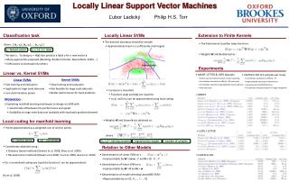
Locally Linear Support Vector Machines Ľubor Ladický Philip H.S. Torr Classification task Locally Linear SVMs Extension to Finite Kernels • The decision boundary should be smooth • Approximately linear in a sufficiently small region • The finite kernel classifier takes the form : • Weights W and b obtained as : Given : { [x1, y1], [x2, y2], … [xn, yn] } xi - feature vector yi {-1, 1} - label • The task is : To design y = H(x) that predicts a label y for a new vector x • Many approaches proposed (Boosting, Random Forests, Neural Nets, SVMs, ..) • SVM seems to dominate the others Experiments • CALTECH-101 (15 samples per class) • Coordinates evaluated on kNN (k = 5) • Approximated Intersection kernel used • Spatial pyramid of BOW features • Coordinates evaluated based on image histograms Linear vs. Kernel SVMs • MNIST, LETTER & USPS datasets • Anchor points obtained using K-means clustering • Coordinates evaluated on kNN (k = 8) (slow part) • Coordinates obtained using weighted inverse distance • Raw data used • Kernel SVMs • Slow training and evaluation • Not feasible for large scale data sets • Better performance for hard problems • Linear SVMs • Fast training and evaluation • Applicable to large scale data sets • Low discriminative power • Curvature is bounded • Functions wi(x) and b(x) are Lipschitz • wi(x) and b(x)can be approximated using local coding • MNIST • Motivation : • Exploiting manifold learning techniques to design an SVM with • Good trade-off between the performance and speed • Scalability to large scale data sets (solvable with stochastic gradient descent) • Weights W and biases b are obtained as : • where Local coding for manifold learning • Points approximated as a weighted sum of anchor points • Coordinates obtained using : • Distance based methods (Gemert et al. 2008, Zhou et al. 2009) • Reconstruction methods (Roweis et al.2000, Yu et al. 2009, Gao et al. 2010) • USPS / LETTER v – anchor points v(x) - coordinates γ [xk, yk] – training samples λ- regularisation weight S – number of samples Relation to Other Models • Generalisation of Linear SVM on x : • representable by W = (ww ..)T and b = (b’ b’ ..)T • Generalisation of linear SVM on γ: • representable by W = 0 andb = w • Generalisation of model selecting Latent(MI) SVM : • Representable by γ= (0, 0, .., 1, .. 0) • CALTECH-101 • For a normalised coding any Lipschitz function f can be approximated : • (Yu et al. 2009)