Download
1 / 25
270 likes | 579 Vues
Direct Numerical Simulation of Transport Phenomena on Pore-space Images. Peyman Mostaghimi, Martin Blunt, Branko Bijeljic 11 th January 2010, Pore-scale project meeting. Flow at pore scale. In petroleum science and engineering, scales of interest may vary from molecular level to a mega level.

E N D
Direct Numerical Simulation of Transport Phenomena on Pore-space Images Peyman Mostaghimi, Martin Blunt, Branko Bijeljic 11th January 2010, Pore-scale project meeting
Flow at pore scale • In petroleum science and engineering, scales of interest may vary from molecular level to a mega level. • The pore scale is of the order of a typical pore which is in the range few microns. Modelling fluid flow at the pore scale can provide a predictive tool for estimating rock and flow properties at larger scales. • One of the most used ways to capture the • morphology of a porous medium as the • main input for pore scale modelling is • micro-CT imaging.
Motivation • Network modelling – the representation of the pore space by an equivalent representation of pores and throats – has been successful: we now understand trends in recovery with wettability and can predict single and multi-phase properties. • However…….the extraction of networks involves ambiguities and there are some cases where the method does not work so well. • Now have direct three-dimensional imaging of pore spaces. • Why not simulate multiphase flow directly on these images?
Micro-CT imaging AND DIRECT SIMULATION Post processing Micro-CT images, a matrix can be generated for a core which shows whether there is a solid inside the voxel or a pore. Zero means that voxel is a pore and one means it is a solid phase. • Two methods to simulate fluid flow in porous media directly without the need for simplified geometries: • - the lattice Boltzmann method (Edo) • - conventional computational fluid dynamics algorithms based on the relevant flow and conservation equations.
Governing equations Conservation of mass: Navier-Stokes equation: Steady-state and incompressible flow:
Dimensionless analysis The dimensionless steady-state Navier-Stokes equation: Reynolds number for flow in porous media: Stokes Equation :
FORMULATION u Equation (u: velocity in x-direction) v Equation (v: velocity in y-direction) w Equation (w: velocity in z-direction) p Equation
Gridding • Marker-and-cell grid: • Existence of solid phase in each grid causes six velocity components be zero in the 3 dimensional models.
Discretized Form The momentum equations can be rewritten as:
SIMPLE algorithm • The SIMPLE (Semi-Implicit Method for pressure-Linked Equations) Algorithm: • 1. Guess the pressure field p* • 2. Solve the momentum equations to obtain u*,v*,w* by algebraic mutigrid solver • 3. Solve the p’ equation (The pressure-correction equation) by algebraic mutigrid solver • 4. p=p*+p’ • 5. Calculate u, v, w from their starred values using the • velocity-correction equations • 6. Solve the discretization equation for other variables, such as • temperature, concentration, and turbulence quantities. • 7. Treat the corrected pressure p as a new guessed pressure p*, • return to step 2, and repeat the whole procedure until a • converged solution is obtained. Storing matrices in CRS and AMG for solving all linear systems of equations.
COMPARISON OF THE Three METHODS FOR BC FOR FLOW BETWEEN TWO INFINITE PARALEL PLATES • first method second method third method
VELOCITY PROFILE FOR FLOW BETWEEN TWO INFINITE PARALEL PLATES • We see non-zero velocity even for one block within the channel and for more than one we see agreement to within machine accuracy with the analytical solution.
DISPERSION MODELLING • When a miscible fluid is injected in a flowing fluid in a saturated porous media, it will spread by various mechanisms including advection and diffusion. • In brief, dispersion is the spread or mixing of flowing fluids due to all these mechanisms. • To model advection term we use stream tracing algorithm and for diffusion we apply random walk method.
STREAMLINE TRACING • Interpolation to estimate the velocity vectors at a point within the grid block The time of flight: • The coordinates of exit location:
Diffusion • Random walking method for both advection and diffusion: advection diffusion Random walking method just for diffusion part of flow :
. . . Diffusion • Gridding: • Resolution:
. . . Particle tracking • Gridding: • Resolution: • Sandpack LV60B
. . . Particle tracking Gridding: Resolution: Sandpack LV60B
. . . Particle tracking • Gridding: • Resolution: • Sandpack LV60B
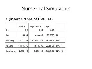
DISPERSION COEFFIEICENT • The average of positions of particles: • Variance of X can be calculated: • And the longitudinal dispersion coefficient: • For showing the importance of diffusion, dispersion is modelled for a range Peclet number: (Bijeljic et al. 2004)
Multiphase flow at the pore scale • Having the interface at different saturations, the flow of each phase can be modelled by the Stokes solver and the relative permeability can be predicted. • Also for reactive transport (Branko), the code can be used to simulate the flow at each time step. Courtesy of MasaProdanovic