Download
1 / 22
220 likes | 421 Vues
Simulation of reactive transport on pore-scale images. Zaki Al Nahari, Branko Bijeljic, Martin Blunt. Motivation. Contaminant transport: Industrial waste remedy Biodegradation of landfills Carbon capture and storage: Acidic brine. Over time, potential dissolution and/or mineral trapping.

E N D
Simulation of reactive transport on pore-scale images Zaki Al Nahari, Branko Bijeljic, Martin Blunt
Motivation • Contaminant transport: • Industrial waste remedy • Biodegradation of landfills • Carbon capture and storage: • Acidic brine. • Over time, potential dissolution and/or mineral trapping. • However…. • Uncertainty in reaction rates • The field <<in the lab. • No fundamental basis to integrate flow, transport and reaction in porous media.
Physical description of reactive transport model Micro-CT scanner uses X-rays to produce a sequence of cross-sectional tomography images of rocks in high resolution (µm) • Place particles on the image • B injected in the first layer • A is placed in the rest of the image Advection along streamlines using a novel formulation accounting for zero flow at solid boundaries. It is based on a semi-analytical approach: no further numerical errors once the flow is computed at cell faces • Geometry • Flow Field • Reactants Injection • Reaction • Transport by Advection • Transport by Diffusion For incompressible laminar flow, Stokes equations Diffusion using random walk. It is a series of spatial random displacements that define the particle transitions by diffusion.
Geometry, Flow , Particle Tracking Particle tracking: Volume placement and front injection Pore space Velocity field Pressure field Particle tracking: Transport and fluid/fluid reaction
Reaction Rate • Bimolecular reaction • A + B → C • The reaction occurs if two conditions are met: • Distance between reactant is less than or equal the diffusive step ( ) • If there is more than one possible reactant, the reaction will be with the nearest reactant. • The probability of reaction (Pr) as a function of reaction rate constant (k) and diffusive step ( ) :
Fluid/fluid reactive transport benchmark experiment by Gramling et al (2002) • Description: • The experiment was conducted by Gramling et al. (2002) • Irreversible Bimolecular reaction • Na2EDTA2- + CuSO4(aq) → CuEDTA2- + 2Na+ + SO42- • A + B → C • The column is filled with grains of cryolite (Na3AlF6) • Reactant A was filled in the column and displaced by B • The change in the colour of solution records the progression of reaction Gramling et al. (2002)
Validation of the Model with benchmark experiment by Gramling et al (2002) Gramling et al. (2002)
Beadpack image used in simulation Pore space Pressure field Velocity field Used beadpack with grain size 100 microns: To have the grain size of 1.3mm as in Gramling et al. need to multiply by 13
Comparison of PDFs of voxel velocities for different beadpack image sizes and resolution 3003beadpack with 26micron resolution can be used
Size of the system in which particles A are initially placed 1 1 1 Image Image 2 Image Image 1 299x(n-1) 300 300 600 598 894 300 299xn 299 Image 1 Image n 0 μm 0 μm 0 μm 0 μm 7774x(n-1)μm 7774xn μm 15548 μm 23244 μm 15600 μm 7774 μm 7800 μm 7800 μm 7800 μm Image 2 Image 3 Image n-1
Product concentration profile at t= 619s - Particle A placed in 5 images
Product concentration profile at t= 619s - Particle A placed in 1 image
Product concentration profile at t= 619s - Particle A placed in 5 images
Product concentration profile at t= 619s - Particle A placed in 10 images
Conclusions • Developed a new particle tracking-based simulator for fluid/fluid reactive transport directly on the pore space of micro-CT images • The simulator is validated by comparison with the bechmark fluid/fluid reactive transport experiments by Gramling et al.(2002) • Capability to study the impact of heterogeneity in pore structure, velocity field, transport and reaction on the physicochemical processes in the subsurface
Acknowledgements: Dr. Branko Bijeljic and Prof. Martin Blunt Emirates Foundation for funding this project Thank you
Validation for bulk reaction • Reaction in a bulk system against the analytical solution: • no porous medium • no flow • Analytical solution for concentration in bulk with no flow. • Number of Voxels: • Case 1: 10×10×10 • Case 2: 20×20×20 • Case 3: 50×50×50 • Number of particles: • A= 100,000 density= 0.8 Np/voxel • B= 50,000 density= 0.4 Np/voxel • Parameters: • Dm= 7.02x10⁻¹¹ m2/s • k= 2.3x10⁹ M-1.s-1 • Time step sizes: • Δt= 10-3 s P= 3.335×10⁻³ • Δt= 10-4 s P= 1.055×10⁻² • Δt= 10-5 s P= 3.335×10⁻²
Case 1: Number of Voxels= 10×10×10 Δt= 10-3 s Δt= 10-4 s Δt= 10-5 s
Case 2: Number of Voxels= 20×20×20 Δt= 10-3 s Δt= 10-4 s Δt= 10-5 s
Case 3: Number of Voxels= 50×50×50 Δt= 10-3 s Δt= 10-4 s