Chapter 9 Comparing Two Groups
Chapter 9 Comparing Two Groups. Learn …. How to Compare Two Groups On a Categorical or Quantitative Outcome Using Confidence Intervals and Significance Tests. Bivariate Analyses. The outcome variable is the response variable


Chapter 9 Comparing Two Groups
E N D
Presentation Transcript
Chapter 9Comparing Two Groups • Learn …. How to Compare Two Groups On a Categorical or Quantitative Outcome Using Confidence Intervals and Significance Tests
Bivariate Analyses • The outcome variable is theresponse variable • The binary variable that specifies the groups is theexplanatory variable
Bivariate Analyses • Statistical methods analyze how the outcome on the response variabledepends on oris explained bythe value of the explanatory variable
Independent Samples • The observations in one sample are independent of those in the other sample • Example: Randomized experiments that randomly allocate subjects to two treatments • Example: An observational study that separates subjects into groups according to their value for an explanatory variable
Dependent Samples • Data are matched pairs – each subject in one sample is matched with a subject in the other sample • Example: set of married couples, the men being in one sample and the women in the other. • Example: Each subject is observed at two times, so the two samples have the same people
Section 9.1 Categorical Response: How Can We Compare Two Proportions?
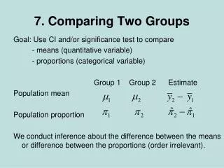
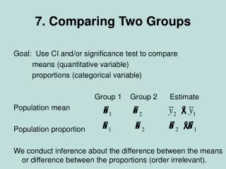
Categorical Response Variable • Inferences compare groups in terms of their population proportions in a particular category • We can compare the groups by the difference in their population proportions: (p1 – p2)
Example: Aspirin, the Wonder Drug • Recent Titles of Newspaper Articles: • “Aspirin cuts deaths after heart attack” • “Aspirin could lower risk of ovarian cancer” • “New study finds a daily aspirin lowers the risk of colon cancer” • “Aspirin may lower the risk of Hodgkin’s”
Example: Aspirin, the Wonder Drug • The Physicians Health Study Research Group at Harvard Medical School • Five year randomized study • Does regular aspirin intake reduce deaths from heart disease?
Example: Aspirin, the Wonder Drug • Experiment: • Subjects were 22,071 male physicians • Every other day, study participants took either an aspirin or a placebo • The physicians were randomly assigned to the aspirin or to the placebo group • The study was double-blind: the physicians did not know which pill they were taking, nor did those who evaluated the results
Example: Aspirin, the Wonder Drug Results displayed in a contingency table:
Example: Aspirin, the Wonder Drug • What is the response variable? • What are the groups to compare?
Example: Aspirin, the Wonder Drug • The response variable is whether the subject had a heart attack, with categories ‘yes’ or ‘no’ • The groups to compare are: • Group 1: Physicians who took a placebo • Group 2: Physicians who took aspirin
Example: Aspirin, the Wonder Drug • Estimate the difference between the two population parameters of interest
Example: Aspirin, the Wonder Drug • p1: the proportion of the population who would have a heart attack if they participated in this experiment and took the placebo • p2: the proportion of the population who would have a heart attack if they participated in this experiment and took the aspirin
Example: Aspirin, the Wonder Drug Sample Statistics:
Example: Aspirin, the Wonder Drug • To make an inference about the difference of population proportions, (p1 – p2), we need to learn about the variability of the sampling distribution of:
Standard Error for Comparing Two Proportions • The difference, , is obtained from sample data • It will vary from sample to sample • This variation is the standard error of the sampling distribution of :
Confidence Interval for the Difference between Two Population Proportions • The z-score depends on the confidence level • This method requires: • Independent random samples for the two groups • Large enough sample sizes so that there are at least 10 “successes” and at least 10 “failures” in each group
Confidence Interval Comparing Heart Attack Rates for Aspirin and Placebo • 95% CI:
Confidence Interval Comparing Heart Attack Rates for Aspirin and Placebo • Since both endpoints of the confidence interval (0.005, 0.011) for (p1- p2) are positive, we infer that (p1- p2) is positive • Conclusion: The population proportion of heart attacks is larger when subjects take the placebo than when they take aspirin
Confidence Interval Comparing Heart Attack Rates for Aspirin and Placebo • The population difference (0.005, 0.011) is small • Even though it is a small difference, it may be important in public health terms • For example, a decrease of 0.01 over a 5 year period in the proportion of people suffering heart attacks would mean 2 million fewer people having heart attacks
Confidence Interval Comparing Heart Attack Rates for Aspirin and Placebo • The study used male doctors in the U.S • The inference applies to the U.S. population of male doctors • Before concluding that aspirin benefits a larger population, we’d want to see results of studies with more diverse groups
Interpreting a Confidence Interval for a Difference of Proportions • Check whether 0 falls in the CI • If so, it is plausible that the population proportions are equal • If all values in the CI for (p1- p2) are positive, you can infer that (p1- p2) >0 • If all values in the CI for (p1- p2) are negative, you can infer that (p1- p2) <0 • Which group is labeled ‘1’ and which is labeled ‘2’ is arbitrary
Interpreting a Confidence Interval for a Difference of Proportions • The magnitude of values in the confidence interval tells you how large any true difference is • If all values in the confidence interval are near 0, the true difference may be relatively small in practical terms
Significance Tests Comparing Population Proportions 1. Assumptions: • Categorical response variable for two groups • Independent random samples
Significance Tests Comparing Population Proportions Assumptions (continued): • Significance tests comparing proportions use the sample size guideline from confidence intervals: Each sample should have at least about 10 “successes” and 10 “failures” • Two–sided tests are robust against violations of this condition • At least 5 “successes” and 5 “failures” is adequate
Significance Tests Comparing Population Proportions 2. Hypotheses: • The null hypothesis is the hypothesis of no difference or no effect: H0: (p1- p2) =0 • Under the presumption that p1= p2, we create a pooled estimate of the common value of p1and p2 • This pooled estimate is
Significance Tests Comparing Population Proportions 2. Hypotheses (continued): Ha: (p1- p2) ≠ 0 (two-sided test) Ha: (p1- p2) < 0 (one-sided test) Ha: (p1- p2) > 0 (one-sided test)
Significance Tests Comparing Population Proportions 3. The test statistic is:
Significance Tests Comparing Population Proportions 4. P-value: Probability obtained from the standard normal table 5. Conclusion: Smaller P-values give stronger evidence against H0 and supporting Ha
Example: Is TV Watching Associated with Aggressive Behavior? • Various studies have examined a link between TV violence and aggressive behavior by those who watch a lot of TV • A study sampled 707 families in two counties in New York state and made follow-up observations over 17 years • The data shows levels of TV watching along with incidents of aggressive acts
Example: Is TV Watching Associated with Aggressive Behavior?
Example: Is TV Watching Associated with Aggressive Behavior? Test the Hypotheses: H0: (p1- p2) = 0 Ha: (p1- p2) ≠ 0 • Using a significance level of 0.05 • Group 1: less than 1 hr. of TV per day • Group 2: at least 1 hr. of TV per day
Example: Is TV Watching Associated with Aggressive Behavior?
Example: Is TV Watching Associated with Aggressive Behavior? • Conclusion: Since the P-value is less than 0.05, we reject H0 • We conclude that the population proportions of aggressive acts differ for the two groups • The sample values suggest that the population proportion is higher for the higher level of TV watching
In 2002, the median net worth was estimated as $89,000 for white households and $6000 for black households. What is the response variable? • Net worth • Households: white or black
In 2002, the median net worth was estimated as $89,000 for white households and $6000 for black households. What is the explanatory variable? • Net worth • Households: white or black
In 2002, the median net worth was estimated as $89,000 for white households and $6000 for black households. • Identify the two groups that are the categories of the explanatory variable. • White and Black households • Net worth and households
In 2002, the median net worth was estimated as $89,000 for white households and $6000 for black households. • The estimated medians were based on a sample of households. Were the samples of white households and black households independent samples or dependent samples? • Independent samples • Dependent samples
Section 9.2 Quantitative Response: How Can We Compare Two Means?
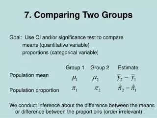
Comparing Means • We can compare two groups on a quantitative response variable by comparing their means
Example: Teenagers Hooked on Nicotine • A 30-month study: • Evaluated the degree of addiction that teenagers form to nicotine • 332 students who had used nicotine were evaluated • The response variable was constructed using a questionnaire called the Hooked on Nicotine Checklist (HONC)
Example: Teenagers Hooked on Nicotine • The HONC score is the total number of questions to which a student answered “yes” during the study • The higher the score, the more hooked on nicotine a student is judged to be
Example: Teenagers Hooked on Nicotine • The study considered explanatory variables, such as gender, that might be associated with the HONC score
Example: Teenagers Hooked on Nicotine • How can we compare the sample HONC scores for females and males? • We estimate (µ1 - µ2) by (x1 - x2): 2.8 – 1.6 = 1.2 • On average, females answered “yes” to about one more question on the HONC scale than males did
Example: Teenagers Hooked on Nicotine • To make an inference about the difference between population means, (µ1 – µ2), we need to learn about the variability of the sampling distribution of:
Standard Error for Comparing Two Means • The difference, , is obtained from sample data. It will vary from sample to sample. • This variation is the standard error of the sampling distribution of :
Confidence Interval for the Difference between Two Population Means • A 95% CI: • Software provides the t-score with right-tail probability of 0.025
Confidence Interval for the Difference between Two Population Means • This method assumes: • Independent random samples from the two groups • An approximately normal population distribution for each group • this is mainly important for small sample sizes, and even then the method is robust to violations of this assumption