Linear Programming (LP) (Chap.29)
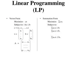
Linear Programming (LP) (Chap.29). Suppose all the numbers below are real numbers. Given a linear function (called objective function ) f ( x 1 , x 2 ,…, x n )= c 1 x 1 + c 2 x 2 +…+ c n x n = j =1 n c j x j . With constraints: j =1 n a ij x j b i for i =1,2,…, m and

Linear Programming (LP) (Chap.29)
E N D
Presentation Transcript
Linear Programming (LP) (Chap.29) • Suppose all the numbers below are real numbers. • Given a linear function (called objective function) • f(x1, x2,…, xn)=c1x1+ c2x2+…+ cnxn=j=1n cjxj. • With constraints: • j=1n aijxj bi for i=1,2,…,m and • xj0 for j=1,2,…,n. (nonnegativity) • Question: find values for x1, x2,…, xn, which maximize f(x1, x2,…, xn). • Or if change bi to bi , then minimize f(x1, x2,…, xn).
LP examples • Political election problem: • Certain issues: building roads, gun control, farm subsidies, and gasoline tax. • Advertisement on different issues • Win the votes on different areas: urban, suburban, and rural. • Goal: minimize advertisement cost to win the majority of each area. (See page 772, (29.6) –(29.10)) • Flight crew schedule, minimize the number of crews: • Limitation on number of consecutive hours, • Limited to one model each month,… • Oil well location decision with maximum of oil output: • A location is associated a cost and payoff of barrels of oil. • Limited budget.
Change a LP problem to standard format • If some variables, such as xi,may not have nonnegativity constraints: • delete xi but introduce two variables xi' and xi'', • Replace each occurrence of xi with xi'-xi''. • Add constraints: xi'0 and xi''0. • There may be equality constraints: • Replace j=1n aijxj =bi with j=1n aijxj bi and j=1n aijxj bi . • Then change j=1n aijxj bi to j=1n -aijxj -bi for minimization or j=1n aijxj bi to j=1n -aijxj -bi for maximization.
Linear program in slack form • Except nonnegativity constraints, all other constraints are equalities. • Change standard form to slack form: • If j=1n aijxj bi, then introduce new variable s, and set: • si= bi - j=1n aijxj and si0. (i=1,2,…,m). • If j=1n aijxj bi, then introduce new variable s, and set: • si= j=1n aijxj -bi and si0. • All the left-hand side variables are called basic variables, whereas all the right-hand side variables are called nonbasic variables. • Initially, s1, s1,…, smbasic variables, x1, x1,…, xnnon-basic variables.
Formatting problems as LPs • (Single pair) Shortest path : • A weighted direct graph G=<V,E> with weighted function w: ER, a source s and a destination t, compute d which is the weight of the shortest path from s to t. • Change to LP: • For each vertex v, introduce a variable xv: the weight of the shortest path from s to v. • Maximize xt with the constraints: • xv xu+w(u,v) for each edge (u,v)E, and xs =0.
Formatting problems as LPs • Max-flow problem: • A directed graph G=<V,E>, a capacity function on each edge c(u,v) 0 and a source s and a sink t. A flow is a function f : VVR that satisfies: • Capacity constraints: for all u,vV, f(u,v) c(u,v). • Skew symmetry: for all u,vV, f(u,v)= -f(v,u). • Flow conservation: for all uV-{s,t}, vVf(u,v)=0, or to say, total flow out of a vertex other s or t is 0, or to say, how much comes in, also that much comes out. • Find a maximum flow from s to t.
Formatting Max-flow problem as LPs • Maximize vVf(s,v) with constraints: • for all u,vV, f(u,v) c(u,v). • for all u,vV, f(u,v)= -f(v,u). • for all uV-{s,t}, vVf(u,v)=0.
Linear Programming (LP) (Chap.29) • Suppose all the numbers below are real numbers. • Given a linear function (called objective function) • f(x1, x2,…, xn)=c1x1+ c2x2+…+ cnxn=j=1n cjxj. • With constraints: • j=1n aijxj bi for i=1,2,…,m and • xj0 for j=1,2,…,n. (nonnegativity) • Question: find values for x1, x2,…, xn, which maximize f(x1, x2,…, xn). • Or if change bi to bi , then minimize f(x1, x2,…, xn).
Linear program in slack form • Except nonnegativity constraints, all other constraints are equalities. • Change standard form to slack form: • If j=1n aijxj bi, then introduce new variable s, and set: • si= bi - j=1n aijxj and si0. (i=1,2,…,m). • If j=1n aijxj bi, then introduce new variable s, and set: • si= j=1n aijxj -bi and si0. • All the left-hand side variables are called basic variables, whereas all the right-hand side variables are called nonbasic variables. • Initially, s1, s1,…, smbasic variables, x1, x1,…, xnnon-basic variables.
The Simplex algorithm for LP • It is very simple • It is often very fast in practice, even its worst running time is not poly. • Illustrate by an example.
An example of Simplex algorithm • Maximize 3x1+x2+2x3 (29.56) • Subject to: • x1+x2+3x3 30 (29.57) • 2x1+2x2+5x3 24 (29.58) • 4x1+x2+2x3 36 (29.59) • x1, x2, x30 (29.60) • Change to slack form: • z= 3x1+x2+2x3 (29.61) • x4=30- x1-x2-3x3 (29.62) • x5=24- 2x1-2x2-5x3(29.63) • x6=36- 4x1-x2-2x3 (29.64) • x1, x2, x3,x4, x5, x6 0
Simplex algorithm steps • Feasible solutions (infinite number of them): • A solution whose values satisfy constraints, in this example, • as long as all of x1, x2, x3,x4, x5, x6 are nonnegative. • basic solution: • set all nonbasic variables to 0 and compute all basic variables • Iteratively rewrite the set of equations such that • No change to the underlying LP problem. • The feasible solutions keep the same. • However the basic solution changes, resulting in a greater objective value each time: • Select a nonbasic variable xe whose coefficient in objective function is positive, • increase value of xe as much as possible without violating any of constraints, • xe is changed to basic and some other variable to nonbasic.
Simplex algorithm example • Basic solution: (x1,x2,x3,x4,x5,x6) =(0,0,0,30,24,36). • The result is z=3 0+0+2 0=0. Not maximum. • Try to increase the value of x1: • z= 3x1+x2+2x3 (29.61) • x4=30- x1-x2-3x3 (29.62) • x5=24- 2x1-2x2-5x3(29.63) • x6=36- 4x1-x2-2x3 (29.64) • 30: x4 will be OK; 12: x5; 9: x6. So only to 9. • Change x1to basic variable by rewriting (29.64) to: • x1=9-x2/4 –x3/2 –x6/4 • Note: x6 becomes nonbasic. • Replace x1 with above formula in all equations to get:
Simplex algorithm example • z=27+x2/4 +x3/2 –3x6/4 (29.67) • x1=9-x2/4 –x3/2 –x6/4 (29.68) • x4=21-3x2/4 –5x3/2 +x6/4 (29.69) • x5=6-3x2/2 –4x3 +x6/2 (29.70) • This operation is called pivot. • A pivot chooses a nonbasic variable, called entering variable, and a basic variable, called leaving variable, and changes their roles. • It can be seen the pivot operation is equivalent. • It can be checked the original solution (0,0,0,30,24,36) satisfies the new equations. • In the example, • x1 is entering variable, and x6 is leaving variable. • x2, x3,x6 are nonbasic, and x1, x4,x5 becomes basic. • The basic solution for this is (9,0,0,21,6,0), with z=27.
Simplex algorithm example • We continue to try to find a new variable whose value may increase. • x6 will not work, since z will decrease. • x2 andx3 are OK. Suppose we select x3. • How far can we increase x3 : • (29.68) limits it to 18, (29.69) to 42/5, (29.70) to 3/2. So rewrite (29.70) to: • x3=3/2-3x2/8 –x5/4+x6/8 • Replace x3 with this in all the equations to get:
Simplex algorithm example • The LP equations: • z=111/4+x2/16 –x5/8 - 11x6/16 (29.71) • x1=33/2- x2/16 +x5/8 - 5x6/16 (29.72) • x3=3/2-3x2/8 –x5/4+x6/8 (29.73) • x4=69/4+3x2/16 +5x5/8-x6/16 (29.74) • The basic solution is (33/4,0,3/2,69/4,0,0) with z=111/4. • Now we can only increase x2. (29,72), (29.73), (29.74) limits x2 to 132,4, respectively. So rewrite (29.73) to x2=4-8x3/3 –2x5/3+x6/3 • Replace in all equations to get:
Simplex algorithm example • LP equations: • z=28-x3/6 –x5/6-2x6/3 • x1=8+x3/6 +x5/6-x6/3 • x2=4-8x3/3 –2x5/3+x6/3 • x4=18-x3/2 +x5/2. • At this point, all coefficients in objective functions are negative. So no further rewrite can be done. In fact, this is the state with optimal solution. • The basic solution is (8,4,0,18,0,0) with objective value z=28. • The original variables are x1, x2, x3 , with values (8,4,0), the objective value of (29.58) =3 8+4+2 0=28.
Simplex algorithm --Pivot N: indices set of nonbasic variables B: indices set of basic variables A: aij b: bi c: ci v: constant coefficient. e: index of entering variable l: index of leaving variable z=v+jNcjxj xi=bi- jNaijxj for iB
Running time of Simplex • Lemma 29.7 (page 803): • Assuming that INITIALIZE-SIMPLEX returns a slack form for which the basic solution is feasible, SIMPLEX either reports that a linear program is unbounded, or it terminates with a feasible solution in at most ( ) iterations. • Feasible solution: a set of values for xi’s which satisfy all constraints. • Unbound: has feasible solutions but does not have a finite optimal objective value. m+n m
Two variable LP problems • Example: • Maximize x1+x2 (29.11) • Subject to: • 4x1- x2 8 (29.12) • 2x1+x2 10 (29.13) • 5x1- 2x2 -2 (29.14) • x1, x2 0 (29.15) • Can be solved by graphical approach. • By prune-and-search approach.
Integer linear program • A linear program problem with additional constraint that all variables must take integral values. • Given an integer mxn matrix A and an integer m-vector b, whether there is an integer n-vector x such that Ax<=b. • this problem is NP-complete. (Prove it??) • However the general linear program problem is poly time solvable.