Robust PCA in Stata
Robust PCA in Stata. Vincenzo Verardi (vverardi@fundp.ac.be) FUNDP (Namur) and ULB (Brussels), Belgium FNRS Associate Researcher. Principal component analysis. PCA, transforms a set of correlated variables into a smaller set of uncorrelated variables (principal components).

Robust PCA in Stata
E N D
Presentation Transcript
Robust PCA in Stata Vincenzo Verardi (vverardi@fundp.ac.be) FUNDP (Namur) and ULB (Brussels), Belgium FNRS AssociateResearcher
Principal component analysis PCA, transforms a set of correlated variables into a smaller set of uncorrelated variables (principal components). For p random variables X1,…,Xp. the goal of PCA is to construct a new set of p axes in the directions of greatest variability. Introduction Robust Covariance Matrix Robust PCA Application Conclusion
Principal component analysis X2 Introduction Robust Covariance Matrix Robust PCA Application Conclusion X1
Principal component analysis X2 Introduction Robust Covariance Matrix Robust PCA Application Conclusion X1
Principal component analysis X2 Introduction Robust Covariance Matrix Robust PCA Application Conclusion X1
Principal component analysis X2 Introduction Robust Covariance Matrix Robust PCA Application Conclusion X1
Principal component analysis Hence, for the first principal component, the goal is to find a linear transformation Y=1 X1+2 X2+..+ p Xp (= TX)such that tha variance of Y (=Var(TX) =T ) is maximal The direction of d is given by the eigenvector correponding to the largest eigenvalue of matrix Σ Introduction Robust Covariance Matrix Robust PCA Application Conclusion
Classical PCA The second vector (orthogonal to the first), is the one that has the second highest variance. This corresponds to the eigenvector associated to the second largest eigenvalue And so on … Introduction Robust Covariance Matrix Robust PCA Application Conclusion
Classical PCA The new variables (PCs) have a variance equal to theircorrespondingeigenvalue Var(Yi)= i for all i=1…p The relative variance explained by each PC isgiven by i / i Introduction Robust Covariance Matrix Robust PCA Application Conclusion
Number of PC How many PC should be considered? Sufficient number of PCs to have a cumulative variance explained that is at least 60-70% of the total Kaiser criterion: keep PCs with eigenvalues >1 Introduction Robust Covariance Matrix Robust PCA Application Conclusion
Drawback PCA PCA is based on the classical covariance matrix which is sensitive to outliers … Illustration: Introduction Robust Covariance Matrix Robust PCA Application Conclusion
Drawback PCA PCA is based on the classical covariance matrix which is sensitive to outliers … Illustration: . set obs 1000 . drawnorm x1-x3, corr(C) . matrix list C c1 c2 c3 r1 1 r2 .7 1 r3 .6 .5 1 Introduction Robust Covariance Matrix Robust PCA Application Conclusion
Drawback PCA Introduction Robust Covariance Matrix Robust PCA Application Conclusion
Drawback PCA Introduction Robust Covariance Matrix Robust PCA Application Conclusion
Drawback PCA Introduction Robust Covariance Matrix Robust PCA Application Conclusion
Minimum Covariance Determinant This drawback can be easily solved by basing the PCA on a robust estimation of the covariance (correlation) matrix. A well suited method for this is MCD that considers all subsets containing h% of the observations (generally 50%) and estimates Σ and µ on the data of the subset associated with the smallest covariance matrix determinant. Intuition … Introduction Robust Covariance Matrix Robust PCA Application Conclusion
Generalized Variance The generalized variance proposed by Wilks (1932), is a one-dimensional measure of multidimensional scatter. It is defined as . In the 2x2 case it is easy to see the underlying idea: Introduction Robust Covariance Matrix Robust PCA Application Conclusion Spread due to covariations Rawbivariatespread
Minimum Covariance Determinant Remember, MCD considers allsubsets containing 50% of the observations … However, if N=200, the number of subsets to consider would be: Solution: use subsampling algorithms … Introduction Robust Covariance Matrix Robust PCA Application Conclusion
Fast-MCD Stata code • The implemented algorithm: • Rousseeuw and Van Driessen (1999) • P-subset • Concentration (sorting distances) • Estimation of robust ΣMCD • Estimation of robust PCA Introduction Robust Covariance Matrix Robust PCA Application Conclusion
P-subset Consider a number of subsets containing (p+1) points (where p is the number of variables) sufficientlylarge to be sure that at least one of the subsets does not contain outliers. Calculate the covariance matrix on each subset and keep the one with the smallest determinant Do some fine tuning to get closer to the global solution Introduction Robust Covariance Matrix Robust PCA Application Conclusion
Number of subsets The minimal number of subsets we need to have a probability (Pr) of having at least one clean if a% of outliers corrupt the dataset can be easily derived: Introduction Robust Covariance Matrix Robust PCA Application Conclusion Contamination: %
Number of subsets The minimal number of subsets we need to have a probability (Pr) of having at least one clean if a% of outliers corrupt the dataset can be easily derived: Introduction Robust Covariance Matrix Robust PCA Application Conclusion Will be the probability that one random point in the dataset is not an outlier
Number of subsets The minimal number of subsets we need to have a probability (Pr) of having at least one clean if a% of outliers corrupt the dataset can be easily derived: Introduction Robust Covariance Matrix Robust PCA Application Conclusion Will be the probability that none of the p random points in a p-subset is an outlier
Number of subsets The minimal number of subsets we need to have a probability (Pr) of having at least one clean if a% of outliers corrupt the dataset can be easily derived: Introduction Robust Covariance Matrix Robust PCA Application Conclusion Will be the probability that at least one of the p random points in a p-subset is an outlier
Number of subsets The minimal number of subsets we need to have a probability (Pr) of having at least one clean if a% of outliers corrupt the dataset can be easily derived: Introduction Robust Covariance Matrix Robust PCA Application Conclusion Will be the probability that there is at least one outlier in each of the N p-subsets considered (i.e. that all p-subsets are corrupt)
Number of subsets The minimal number of subsets we need to have a probability (Pr) of having at least one clean if a% of outliers corrupt the dataset can be easily derived: Introduction Robust Covariance Matrix Robust PCA Application Conclusion Will be the probability that there is at least one clean p-subset among the N considered
Number of subsets The minimal number of subsets we need to have a probability (Pr) of having at least one clean if a% of outliers corrupt the dataset can be easily derived: Introduction Robust Covariance Matrix Robust PCA Application Conclusion Rearranging we have:
Concentration steps The preliminary p-subset step allowed to estimate a preliminary Σ* and μ* Calculate Mahalanobis distances using Σ* and μ*for all individuals Mahalanobis distances, are defined as . MD are distributed as for Gaussian data. Introduction Robust Covariance Matrix Robust PCA Application Conclusion
Concentration steps The preliminary p-subset step allowed to estimate a preliminary Σ* and μ* Calculate Mahalanobis distances using Σ* and μ*for all individuals Sort individuals according to Mahalanobis distances and re-estimate Σ* and μ* using the first 50% observations Repeat the previous step till convergence Introduction Robust Covariance Matrix Robust PCA Application Conclusion
RobustΣin Stata In Stata, Hadi’s method is available to estimate a robust Covariance matrix Unfortunately it is not very robust The reason for this is simple, it relies on a non-robust preliminary estimation of the covariance matrix Introduction Robust Covariance Matrix Robust PCA Application Conclusion
Hadi’s Stata code • Compute a variant of MD • Sort individuals according to . Use the subset with the first p+1 points to re-estimate μ and Σ. • Compute MD and sort the data. • Check if the first point out of the subset is an outlier. If not, add this point to the subset and repeat steps 3 and 4. Otherwise stop. Introduction Robust Covariance Matrix Robust PCA Application Conclusion
Fast-MCD vs hadimvo clear set obs 1000 local b=sqrt(invchi2(5,0.95)) drawnorm x1-x5 e replace x1=invnorm(uniform())+5 in 1/100 mcd x*, outlier gen RD=Robust_distance hadimvo x*, gen(a b) p(0.5) scatter RD b, xline(`b') yline(`b') Introduction Robust Covariance Matrix Robust PCA Application Conclusion
Illustration Fast-MCD Introduction Robust Covariance Matrix Robust PCA Application Conclusion Hadi
PCA withoutoutliers Introduction Robust Covariance Matrix Robust PCA Application Conclusion
PCA withoutoutliers Introduction Robust Covariance Matrix Robust PCA Application Conclusion
PCA withoutliers Introduction Robust Covariance Matrix Robust PCA Application Conclusion
PCA withoutliers Introduction Robust Covariance Matrix Robust PCA Application Conclusion
PCA withoutliers Introduction Robust Covariance Matrix Robust PCA Application Conclusion
Robust PCA withoutliers Introduction Robust Covariance Matrix Robust PCA Application Conclusion
Robust PCA withoutliers Introduction Robust Covariance Matrix Robust PCA Application Conclusion
Robust PCA withoutliers Introduction Robust Covariance Matrix Robust PCA Application Conclusion
Application: rankings of Universities QUESTION: Can a single indicator accurately sum up research excellence? GOAL: Determine the underlying factors measured by the variables used in the Shanghai ranking Principal component analysis Introduction Robust Covariance Matrix Robust PCA Application Conclusion
ARWU variables Alumni: Alumni recipients of the Nobel prize or the Fields Medal; Award: Current faculty Nobel laureates and Fields Medal winners; HiCi : Highly cited researchers N&S: Articles published in Nature and Science; PUB: Articles in the Science Citation Index-expanded, and the Social Science Citation Index; Introduction Robust Covariance Matrix Robust PCA Application Conclusion
PCA analysis (on TOP 150) Introduction Robust Covariance Matrix Robust PCA Application Conclusion
PCA analysis (on TOP 150) Introduction Robust Covariance Matrix Robust PCA Application Conclusion
PCA analysis (on TOP 150) Introduction Robust Covariance Matrix Robust PCA Application Conclusion
ARWU variables The first component accounts for 68% of the inertia and is given by: Φ1=0.42Al.+0.44Aw.+0.48HiCi+0.50NS+0.38PUB Introduction Robust Covariance Matrix Robust PCA Application Conclusion
Robust PCA analysis (on TOP 150) Introduction Robust Covariance Matrix Robust PCA Application Conclusion
Robust PCA analysis (on TOP 150) Introduction Robust Covariance Matrix Robust PCA Application Conclusion
Robust PCA analysis (on TOP 150) Introduction Robust Covariance Matrix Robust PCA Application Conclusion