Structural Data Analysis of Sand Brook Syncline
40 likes | 72 Vues
Analyze structural data from 8 field stations in the syncline. Use software to generate diagrams of bedding and fractures. Follow instructions to create a GIF image for presentation.

Structural Data Analysis of Sand Brook Syncline
E N D
Presentation Transcript
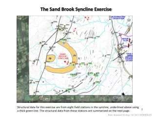
The Sand Brook Syncline Exercise Structural data for this exercise are from eight field stations in the syncline, underlined above using a thick green line. The structural data from these stations are summarized on the next page. Rider Structural Geology 310 2012 GCHERMAN
There are 8 bedding readings and 24 fracture readings in the Excel file. The dip azimuth has already been calculated for you. Copy and past the DIP and DIPAZM data into Notepad if you using windows or a text editor using a Mac. Save the files for input into GEOrient or other histogram and Stereonet software of your choice. The goal is to generate a GIF image of the bedding and fracture results with one diagram that includes circular histograms, equal-angle stereonet projection with density contours, and equal-angle cyclographic plots of the bedding and fractures, like we practiced in class, and that is demonstrated on the following page. Rider Structural Geology 310 2012 GCHERMAN
The trial version of GEOrient allows you to plot three windows. Go through the routine twice, once for beds, and once for fractures, capture the results, and embed them in a MS-Word (doc) file or MS PowerPoint file. There is more on the next page. Rider Structural Geology 310 2012 GCHERMAN
Be sure to activate the Girdle Panel to plot the Beta axis on the cyclographic plot. Take note of it, and compare it to the trend of the fold axis on the map in page one. Notice that stats for the four girdles in the fracture stereonet on the previous page are included. After deriving the dominant planes based on the contours, go to the Edit command in the top menu bar, and select <Recalculate Statistics> in order to display the girdle results on the plot before you capture it. The ‘N’ is placed at the top of each plot using the text editor inside MS-Paint. The notation about the LOWER HEMISPHERE EQUAL ANGLE PLOT is also done with the text editor in Paint. It’s OK to capture and embed two images , one above the other, but it’s best to combine the images, by enlarging the image canvas using the graphics software (for example, MS Paint), then cutting & pasting the 2nd image below the first it so that you end up with just one image. Email me the results before start of next class, preferably by Monday. Rider Structural Geology 310 2012 GCHERMAN