1 / 26

Figure 3-1 (p. 162) ROC for the Z-transform of ( a ) ß n u ( n ); ( b ) ß n u (- n -1).

Figure 3-1 (p. 162) ROC for the Z-transform of ( a ) ß n u ( n ); ( b ) ß n u (- n -1). Figure 3-2 (p. 164) ROC for the Z-transform of the sequence 2 n u ( n ) + (-3) n u (- n -1). Figure 3-3 (p. 168). Figure 3-4 (p. 179) The stability triangle.

bran
Télécharger la présentation

Figure 3-1 (p. 162) ROC for the Z-transform of ( a ) ß n u ( n ); ( b ) ß n u (- n -1).

An Image/Link below is provided (as is) to download presentation Download Policy: Content on the Website is provided to you AS IS for your information and personal use and may not be sold / licensed / shared on other websites without getting consent from its author. Content is provided to you AS IS for your information and personal use only. Download presentation by click this link. While downloading, if for some reason you are not able to download a presentation, the publisher may have deleted the file from their server. During download, if you can't get a presentation, the file might be deleted by the publisher.

E N D

Presentation Transcript


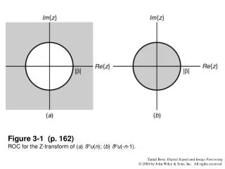
  1. Figure 3-1 (p. 162)ROC for the Z-transform of (a) ßnu(n); (b) ßnu(-n-1).

  2. Figure 3-2 (p. 164)ROC for the Z-transform of the sequence 2nu(n) + (-3)nu(-n-1).

  3. Figure 3-3 (p. 168)

  4. Figure 3-4 (p. 179)The stability triangle.

  5. Figure 3-5 (p. 183)Phase response of a double delay.

  6. Figure 3-6 (p. 183)Typical LPF magnitude response.

  7. Figure 3-7 (p. 184)Examples of FIR filter impulse responses; (a) FIR-I; (b) FIR-II; (c) FIR-III; (d) FIR IV.

  8. Figure 3-8 (p. 187)Responses of FIR-I filter in Example 3.13.

  9. Figure 3-9 (p. 188)Responses of FIR-II filter in Example 3.13

  10. Figure 3-10 (p. 189)Responses of FIR-III filter in Example 3.13.

  11. Figure 3-11 (p. 190)Responses of FIR-IV filter in Example 3.13.

  12. Figure 3-12 (p. 190)Possible zero positions for a linear phase FIR filter. The alphabets refer to the zeros that appear together.

  13. Figure 3-13 (p. 192)Second-order Direct Form II filters.

  14. Figure 3-14 (p. 196)Illustration of the overlap-add method.

  15. Figure 3-15 (p. 198)Illustration of the overlap-save method.

  16. Figure 3-16 (p. 200)First-order Goertzel filter.

  17. Figure 3-17 (p. 201)Second-order Goertzel filter to compute X(k).

  18. Figure 3-18 (p. 202)Sample contours for the CZT.

  19. Figure 3-19 (p. 203)The CZT algorithm.

  20. Figure 3-20 (p. 205)(a) 2d(n2)u(n1, n2); (b) ROC.

  21. Figure 3-21 (p. 206)(a) u(n1, n2); (b) ROC.

  22. Figure 3-22 (p. 206)(a) u2d(n1)2d(n1-n2); (b) ROC.

  23. Figure 3-23 (p. 207)ROC of the Z-transform of an1bn2u(-n1, -n2).

  24. Figure 3-24 (p. 213)Efficient computation of condition I.2 in Huang’s theorem.

  25. Figure P3-1 (p. 221)

  26. Figure P3-2 (p. 222)

More Related