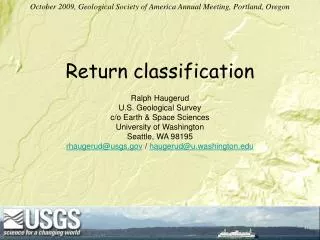
Return classification
October 2009, Geological Society of America Annual Meeting, Portland, Oregon. Return classification. Ralph Haugerud U.S. Geological Survey c/o Earth & Space Sciences University of Washington Seattle, WA 98195 rhaugerud@usgs.gov / haugerud@u.washington.edu.

Return classification
E N D
Presentation Transcript
October 2009, Geological Society of America Annual Meeting, Portland, Oregon Return classification Ralph Haugerud U.S. Geological Survey c/o Earth & Space Sciences University of Washington Seattle, WA 98195 rhaugerud@usgs.gov / haugerud@u.washington.edu
A lidar point cloud—pure XYZ position profile view 10-ft thick slice 100 ft No vertical exaggeration O 1st return X 2nd return
1 km ground pointsidentified by semi-automatic processing all surveyed points Nookachamps Creek, east of Mount Vernon, Washington
What is ground? • Ground is smooth • despiking, iterative linear interpretation algorithms • Ground is continuous (single-valued) • No-multiples algorithm • Ground is lowest surface in vicinity • Block-minimum algorithms
Ground is smooth • despike algorithm flag all points as ground repeat build TIN (triangulated irregular network) of ground points identify points that define strong positive curvatures flag identified points as not-ground until no or few points are flagged
Start with mixed ground and canopy returns (e.g. last-return data), build TIN
Despike algorithm • It works • It’s automatic • Cheap(!) • All assumptions explicit • It can preserve breaklines • It appears to retain more ground points than other algorithms
Despike algorithm • Removes some corners • Sensitive to negative blunders • Computationally intensive • Makes rough surfaces • Real? Measurement error? Misclassified vegetation? Cross-section of highway cut
Ground is continuous (i.e., single-valued) • No-multiples algorithm Multiple returns from pulse Single return from pulse
No-multiples algorithms • Fast • Identify open areas • Hopeless in woods
Ground is lowest surface in vicinityblock minimum algorithms • Computationally rapid with raster processing • Tweedy texture • Biased low on slopes • Appropriate block size is inversely proportional to penetration rate • Requires human intervention to adjust block size • Implicit assumption that ground is horizontal (Successful users of block-minimum algorithms work in flat places)
In the real world… • Almost all return classification is done with proprietary codes • Successful classification uses a mix of • Sophisticated code • Skilled human • To adjust code parameters • To identify and remedy problems • Let somebody else do it! and then carefully check their work • We have no useful metrics for accuracy of return classification
The solution • LAS format • Sponsored by surveying industry, esp. ASPRS (American Society for Photography and Remote Sensing) The problem • Data are voluminous and mostly numeric • Binary formats rule! • A standard file format leads to better tools
LAS 1.0 (May 2003) • Public header block • Data set identifiers • Flight day, year • # records • Data offsets and scale factors • Variable length records • Stuff (projection info, …) • Point records
LAS 1.0 (cont.) • Point data format 0 • Point data format 1 • Adds GPS time as DOUBLE (8 byte floating point number)
LAS 1.1 (March 2005) • Header • modified to better identify data that are not direct-from-sensor • Point data • Classification field becomes mandatory • Standard classification values
LAS 1.2 (September 2008) • Complete time stamp on each point record • GPS second + GPS week OR • POSIX time • Per-point image data (RGB), via new point record types
LAS 1.3 (July 2009) • New point data record types to store waveform data • Modifications to header to store pointer to start of waveform data • Flag for files of synthetically-generated data
Tools for LAS files • Fusion • ArcGIS as of 9.3, LAS 1.0, 1.1 … • liblas (http://liblas.org) LAS 1.0, 1.1, 1.2 • Command-line utilities • C/C++ code library • APIs for Python, .Net/Mono • pylas.py(http://code.google.com/p/pylas/) LAS 1.0, 1.1
What should a data set include? • Report of Survey • All-return point files • Ground points only • Bare-earth raster • First return (highest-hit) raster • Images • Contours • FGDC metadata italics indicate optional elements
Report of Survey • .pdf or .doc or .odt file—or paper! • Data provider, area surveyed, when surveyed, instrument used, processing software and methods, … • Spatial reference framework • Data provider’s report on data quality • Naming, formats, spatial organization of data files Looks a lot like metadata (it is), but in an older and more human-friendly format. The Report of Survey and FGDC metadata commonly have significantly different content. This is a problem.
All-return point files • LAS binary files • Complete time stamp (LAS 1.2+) much better • Organized by tile or by swath Ground points only • Easily(!) extracted from all-return point files, so why bother? • A convenience for AutoCAD community
Bare-earth raster • Format • Many possibilities, ESRI grid is preferable (discuss) • XY resolution (cell size) • Should be a function of return density: ± 1 ground return per cell • Typically in range 2 ft – 5 m • Z resolution • FLOATING POINT! • integer Z requires half the file size, but is almost useless • What about TINs?
First return (highest-hit) raster • Derived shaded-relief image looks like an orthophoto, but with more contrast • 1st-return – bare-earth = buildings, forest • Two ways to construct: • Sample interpolated (TIN?) surface of 1st returns • Bin 1st returns and take highest value in each cell; some cells have NODATA • Better tree and building heights • Can easily see NODATA areas to assess survey completeness
Image files (optional) • Hillshade • Make your own! • Intensity (from 1st returns or ground returns) • A monochromatic low-resolution orthophoto, captured with an active sensor (not dependent on ambient illumination) • RGB orthophotos • A bad idea: drives up cost of lidar by limiting acquisition to mid-day hours
Contours (optional) • You can make your own • See ArcGIS script CartoContours.py • A significant amount of work • Why do you want contours? • Most all analysis is easier with raster (grid) or TIN
FGDC metadata • See recommendations in A proposed specification for lidar surveys in the Pacific Northwest (PSLC website, also included in course materials)