By: Ryan Winters and Cameron Kerst
80 likes | 389 Vues
The Canadian Lynx vs. the Snowshoe Hare: The Predator-Prey Relationship and the Lotka-Volterra Model. By: Ryan Winters and Cameron Kerst. Photo Courtesy of http://taggart.glg.msu.edu/bs110/lynx1.gif. An Overview. The Canadian Lynx population fluctuates based upon the Snowshoe Hare population

By: Ryan Winters and Cameron Kerst
E N D
Presentation Transcript
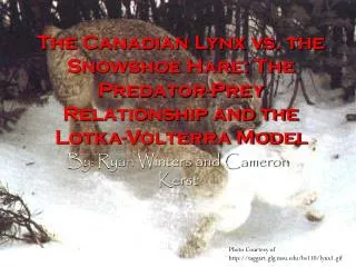
The Canadian Lynx vs. the Snowshoe Hare: The Predator-Prey Relationship and the Lotka-Volterra Model By: Ryan Winters and Cameron Kerst Photo Courtesy of http://taggart.glg.msu.edu/bs110/lynx1.gif
An Overview • The Canadian Lynx population fluctuates based upon the Snowshoe Hare population • Share a common habitat in the Boreal forests of Canada • All data comes from records of the Hudson Bay fur company
Background of the Lotka-Volterra Model • Developed Simultaneously by Alfred J. Lotka and Vito Volterra • Volterra, an Italian professor of math, developed the model while trying to explain his son’s observations of fish predators. • Lotka, a chemist, demographer ecologist and mathematician, addressed the model in his book ElementsofPhysical Biology.
Explaining the Model dH= aH(t)-bH(t)L(t) dL= cH(t)L(t)-eL(t) dt • dH/dt is Malthusian, depends : aH(t) • extension of the basic Verhulst (logistic) Model • Outputs rate at which the respective population in changing at time t • a=intrinsic rate of Hare population increase (births) • b=predation rate coefficient • c=reproduction rate of predators per 1 prey eaten • e=predator mortality rate dt
Applying the Data • We chose values for our coefficients that best fit our population data graph • Also initial conditions were taken under consideration in order to most accurately depict our original data • This yielded these rate equations H’=0.7R(t)-1.25R(t)L(t) L’=R(t)L(t)-L(t) a=0.7 b=1.25 c=1 e=1
IVP and the Model • After finding our rate equations we then formed an IVP with an initial conditions and rate equations • We used our coefficients that we found and used Euler’s Method to compare our model with the actual data I.C.= H(1900)=3* L(1900)=.4* *Population in thousands R.E.= H’= aH(t)-bH(t)L(t) L’= cH(t)L(t)-eL(t)
Works Consulted • Works Consulted: • Lotka, Alfred J. ElementsofPhysicalBiology. • Mahaffy, Joseph M. “Lotka-Volterra Models.” San Diego State University: 2000. http://www- rohan.sdsu.edu/~jmahaffy/courses/f00/math122/lectures/qual_de2/qualde2.html • McKelvey, Steve. “Lotka-Volterra Two Species Model.” <http://www.stolaf.edu/people/mckelvey/envision.dir/lotka-volt.html > • Sharov, Alexei. “Lotka-Volterra Model.” 01/12/1996. < http://www.gypsymoth.ento.vt.edu/~sharov/PopEcol/lec10/lotka.html > • “Vito Voltera.” School of Mathematics and Statistics, University of St. Andrews, Scotland. December 1996. < http://www-groups.dcs.st- and.ac.uk/~history/Mathematicians/Volterra.html > • “Alfred J. Lotka.” Wikipedia. • <http://www.stolaf.edu/people/mckelvey/envision.dir/lotka-volt.html > 12/01/2005
The End Thank You!!!
