QG Analysis: System Evolution
QG Analysis: System Evolution. QG Analysis. QG Theory Basic Idea Approximations and Validity QG Equations / Reference QG Analysis Basic Idea Estimating Vertical Motion QG Omega Equation: Basic Form QG Omega Equation: Relation to Jet Streaks QG Omega Equation: Q-vector Form

QG Analysis: System Evolution
E N D
Presentation Transcript
QG Analysis: System Evolution M. D. Eastin
QG Analysis • QG Theory • Basic Idea • Approximations and Validity • QG Equations / Reference • QG Analysis • Basic Idea • Estimating Vertical Motion • QG Omega Equation: Basic Form • QG Omega Equation: Relation to Jet Streaks • QG Omega Equation: Q-vector Form • Estimating System Evolution • QG Height Tendency Equation • Diabatic and Orographic Processes • Evolution of Low-level Cyclones • Evolution of Upper-level Troughs M. D. Eastin
QG Analysis: Basic Idea • Forecast Needs: • The public desires information regarding temperature, humidity, precipitation, • and wind speed and direction up to 7 days in advance across the entire country • Such information is largely a function of the evolving synoptic weather patterns • (i.e., surface pressure systems, fronts, and jet streams) • Forecast Method: • Kinematic Approach: Analyze current observations of wind, temperature, and moisture fields • Assume clouds and precipitation occur when there is upward motion • and an adequate supply of moisture • QG theory • QG Analysis: • Vertical Motion: Diagnose synoptic-scale vertical motion from the observed • distributions of differential geostrophic vorticity advection • and temperature advection • System Evolution: Predict changes in the local geopotential height patterns from • the observed distributions of geostrophic vorticity advection • and differential temperature advection M. D. Eastin
QG Analysis: A Closed System of Equations • Recall: Two Prognostic Equations –Two Unknowns: • We defined geopotential height tendency (X) and then expressed geostrophic vorticity (ζg) • and temperature (T) in terms of the height tendency. M. D. Eastin
QG Analysis: System Evolution • The QG Height Tendency Equation: • We can also derive a singleprognosticequation for Xby combining our modified • vorticity and thermodynamic equations (the height-tendency versions): • To do this, we need to eliminate the vertical motion (ω) from both equations • Step 1: Apply the operator to the thermodynamic equation • Step 2: Multiply the vorticity equation by • Step 3: Add the results of Steps 1 and 2 • After a lot of math, we get the resulting prognostic equation…… Vorticity Equation Adiabatic Thermodynamic Equation M. D. Eastin
QG Analysis: System Evolution • The QG Height Tendency Equation: • This is (2.32) in the Lackmann text • This form of the equation is not very intuitive since we transformed geostrophic • vorticity and temperature into terms of geopotential height. • To make this equation more intuitive, let’s transform them back… M. D. Eastin
QG Analysis: System Evolution • The BASICQG Height Tendency Equation: • Term ATerm BTerm C • To obtain an actual value for X(the ideal goal), we would need to compute the • forcing terms (Terms B and C) from the three-dimensional wind and temperature fields, • and then invert the operator in Term A using a numerical procedure, called “successive • over-relaxation”, with appropriate boundary conditions • This is NOT a simple task (forecasters never do this)….. • Rather, we can infer the sign and relative magnitude of Xsimple inspection • of the three-dimensional absolute geostrophic vorticity and temperature fields • (forecasters do this all the time…) • Thus, let’s examine the physical interpretation of each term…. M. D. Eastin
QG Analysis: System Evolution • The BASIC QG Height Tendency Equation: • Term ATerm BTerm C • Term A: Local Geopotential Height Tendency • This term is our goal – a qualitative estimate of the synoptic-scale • geopotential height change at a particular location • For synoptic-scale atmospheric waves, this term is proportional to –X • Thus, if we incorporate the negative sign into our physical interpretation, • we can just think of this term as local geopotential height change M. D. Eastin
QG Analysis: System Evolution • The BASIC QG Height Tendency Equation: • Term ATerm BTerm C • Term B: Geostrophic Advection of Absolute Vorticity (Vorticity Advection) • Recall for a Single Pressure Level: • Positive vorticity advection (PVA) PVA → • causes local vorticity increases • From our relationship between ζg and χ, we know that PVA is equivalent to: • therefore: PVA → or, since: PVA → • Thus, we know that PVAat a single level leads toheight falls • Using similar logic, NVA at a single level leads to height rises M. D. Eastin
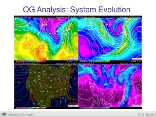
QG Analysis: System Evolution The BASIC QG Height Tendency Equation: Term B: Geostrophic Advection of Absolute Vorticity (Vorticity Advection) Initial Time Trough Axis Initial Time Full-Physics Model Analysis NVA Expect Height Rises PVA Expect Height Falls Expect the trough to move east M. D. Eastin
QG Analysis: System Evolution The BASIC QG Height Tendency Equation: Term B: Geostrophic Advection of Absolute Vorticity (Vorticity Advection) 12 Hours Later Trough Axis Trough Axis Initial Time Generally consistent with expectations! M. D. Eastin
QG Analysis: System Evolution • The BASIC QG Height Tendency Equation: • Term B: Geostrophic Advection of Absolute Vorticity (Vorticity Advection) • Generally Consistent…BUT…Remember! • Only evaluated one level (500mb) → should evaluate multiple levels • Used full wind and vorticity fields → should use geostrophic wind and vorticity • Mesoscale-convective processes → QG focuses on only synoptic-scale (small Ro) • Condensation / Evaporation → neglected diabatic processes • Did not consider differential temperature (thermal) advection (Term C)!!! • Application Tips: • Often the primary forcing in the upper troposphere (500 mb and above) • Term is equal to zero at local vorticity maxima / minima • If the vorticity maxima / minima are collocated with trough / ridge axes, • (which is often the case) this term cannot change system strength by • increasing or decreasing the amplitude of the trough / ridge system • Thus, this term is often responsible for system motion [more on this later…] M. D. Eastin
QG Analysis: System Evolution • The BASIC QG Height Tendency Equation: • Term ATerm BTerm C • Term C: Vertical Derivative of Geostrophic Temperature Advection • (Differential Thermal Advection) • Consider a three layer atmosphere where the warm air advection (WAA) is • strongest in the upper layer • The greater temperature increase aloft will produce the greatest thickness increase • in the upper layer and lower the pressure surfaces (or heights) in the lower levels • Therefore an increase in WAA advectionwith height leads to height falls Z-top Height Falls occur below the level of maximum WAA WAA ΔZ ΔZ increases Z-400mb WAA Z-700mb WAA Z-bottom M. D. Eastin
QG Analysis: System Evolution • The BASIC QG Height Tendency Equation: • Term ATerm BTerm C • Term C: Vertical Derivative of Geostrophic Temperature Advection • (Differential Thermal Advection) • Possible height fall scenarios: Strong WAA in upper levels • Weak WAA in lower levels • WAA in upper level • CAA in lower levels • No temperature advection in upper levels • CAA in lower levels • Weak CAA in upper levels • Strong CAA in lower levels M. D. Eastin
QG Analysis: System Evolution • The BASIC QG Height Tendency Equation: • Term ATerm BTerm C • Term C: Vertical Derivative of Geostrophic Temperature Advection • (Differential Thermal Advection) • Consider a three layer atmosphere where the warm air advection (CAA) is • strongest in the upper layer • The greater temperature increase aloft will produce the greatest thickness increase • in the upper layer and lower the pressure surfaces (or heights) in the lower levels • Therefore an increase in CAA advectionwith heightleads to height rises Z-top ΔZ decreases Height rises occur below the level of maximum CAA CAA ΔZ Z-400mb CAA Z-700mb CAA Z-bottom M. D. Eastin
QG Analysis: System Evolution • The BASIC QG Height Tendency Equation: • Term ATerm BTerm C • Term C: Vertical Derivative of Geostrophic Temperature Advection • (Differential Thermal Advection) • Possible height risescenarios: Strong CAA in upper levels • Weak CAA in lower levels • CAA in upper level • WAAin lower levels • No temperature advection in upper levels • WAA in lower levels • Weak WAA in upper levels • Strong WAA in lower levels M. D. Eastin
QG Analysis: System Evolution The BASIC QG Height Tendency Equation: Term C: Vertical Derivative of Geostrophic Temperature Advection (Differential Thermal Advection) Initial Time 850 mb Initial Trough Axis Full-Physics Model Analysis Strong WWA Weaker WAA aloft (not shown) Expect Height Rises Strong CAA Weaker CAA aloft (not shown) Expect Height Falls M. D. Eastin
QG Analysis: System Evolution The BASIC QG Height Tendency Equation: Term C: Vertical Derivative of Geostrophic Temperature Advection (Differential Thermal Advection) 12 Hours Later 850 mb Initial Trough Axis Generally consistent with expectations! Ridge ”rose” slightly Trough “deepened” M. D. Eastin
QG Analysis: System Evolution • The BASIC QG Height Tendency Equation: • Term C:Vertical Derivative of Geostrophic Temperature Advection • (Differential Thermal Advection) • Generally Consistent…BUT…Remember! • Used full wind field → should use geostrophic wind • Only evaluated one level (850mb) → should evaluate multiple levels/layers** • Mesoscale-convective processes → QG focuses on only synoptic-scale (small Ro) • Condensation / Evaporation → neglected diabatic processes • Did not consider vorticity advection (Term B)!!! • Application Tips: • Often the primary forcing in the lower troposphere (below 500 mb) • Term is equal to zero at local temperature maxima / minima • Since the temperature maxima / minima are often located between the • trough / ridge axes, significant temperature advection (or height changes) • can occur at the axes and thus amplify the system intensity M. D. Eastin
QG Analysis: System Evolution The BASIC QG Height Tendency Equation: Term C:Vertical Derivative of Geostrophic Temperature Advection (Differential Thermal Advection) Important: You should evaluate the vertical structure of temperature advection!!! M. D. Eastin
QG Analysis: System Evolution The BASIC QG Height Tendency Equation: Term C:Vertical Derivative of Geostrophic Temperature Advection (Differential Thermal Advection) Important: You should evaluate the vertical structure of temperature advection!!! N-S Cross-section of Temperature Advection WAA = Warm Colors CAA = Cool Colors M. D. Eastin
QG Analysis: System Evolution • The BASIC QG Omega Equation: • Application Tips: • Remember the underlying assumptions!!! • You must consider the effects of bothTerm B and Term C at multiple levels!!! • If the vorticity maxima/minimaare not collocated with trough/ridge axes, then Term B will contribute to system intensity change and motion • If the vorticity advection patterns change with height, expect the system “tilt” to change with time (become more “tilted” or more “stacked”) • If differential temperature advection is large (small), then expect Term C to produce large (small) changes in system intensity • Opposing expectations from the two terms at a given location will weaken • the total vertical motion (and complicate the interpretation)!!! • The QG height-tendency equation is a prognosticequation: • Can be used to predict the future pattern of geopotential heights • Diagnose the synoptic–scale contribution to the height field evolution • Predict the formation, movement, and evolution of synoptic waves M. D. Eastin
References Bluestein, H. B, 1993: Synoptic-Dynamic Meteorology in Midlatitudes. Volume I: Principles of Kinematics and Dynamics. Oxford University Press, New York, 431 pp. Bluestein, H. B, 1993: Synoptic-Dynamic Meteorology in Midlatitudes. Volume II: Observations and Theory of Weather Systems. Oxford University Press, New York, 594 pp. Charney, J. G., B. Gilchrist, and F. G. Shuman, 1956: The prediction of general quasi-geostrophic motions. J. Meteor., 13, 489-499. Durran, D. R., and L. W. Snellman, 1987: The diagnosis of synoptic-scale vertical motionin an operational environment. Weather and Forecasting, 2, 17-31. Hoskins, B. J., I. Draghici, and H. C. Davis, 1978: A new look at the ω–equation. Quart. J. Roy. Meteor. Soc., 104, 31-38. Hoskins, B. J., and M. A. Pedder, 1980: The diagnosis of middle latitude synoptic development. Quart. J. Roy. Meteor. Soc., 104, 31-38. Lackmann, G., 2011: Mid-latitude Synoptic Meteorology – Dynamics, Analysis and Forecasting, AMS, 343 pp. Trenberth, K. E., 1978: On the interpretation of the diagnostic quasi-geostrophic omega equation. Mon. Wea. Rev., 106, 131-137. M. D. Eastin